What is Bayesian classification?
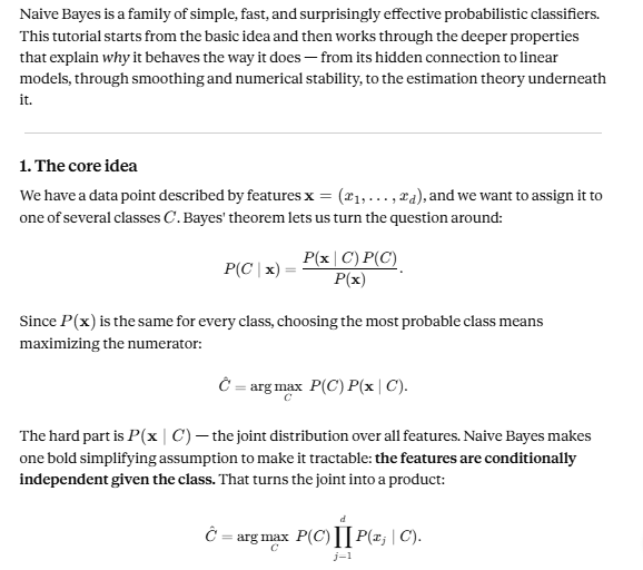
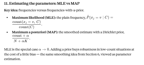
Bayesian classification is a probabilistic approach to predicting the class of a data instance based on Bayes’ theorem. Rather than committing to a single hard rule, it reasons about how likely each class is given the observed features, and assigns the instance to the most probable one. Formally, it computes the posterior probability P(C | X) = [P(X | C) · P(C)] / P(X), where P(C) is the prior (how common the class is before seeing any evidence), P(X | C) is the likelihood (how well the class explains the observed features), and P(X) is the evidence (a normalizing term common to all classes). The classifier then selects the class with the highest posterior — the maximum a posteriori (MAP) decision, which reduces to a maximum likelihood choice when all classes are equally likely.
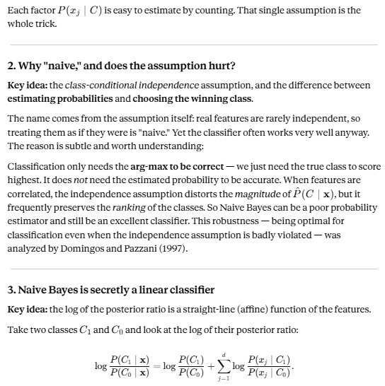
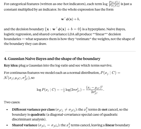
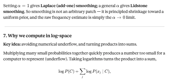
The most widely used form is the Naïve Bayes classifier, which makes one simplifying assumption: that features are conditionally independent given the class. This lets the likelihood factorize into a simple product of per-feature probabilities, making the method fast and effective even with limited training data. Categorical features are handled through frequency counts, with Laplace smoothing applied to avoid zero probabilities, while continuous features are modelled with a distribution such as the Gaussian density, using each class’s mean and variance (Gaussian Naïve Bayes). Despite the “naïve” independence assumption rarely holding exactly, the method performs remarkably well in practice — powering applications like spam filtering, text and document classification, and medical diagnosis — and serves as the foundation for richer probabilistic models such as Bayesian belief networks.
Points to remember
Bayesian Classifier(Continous Values)
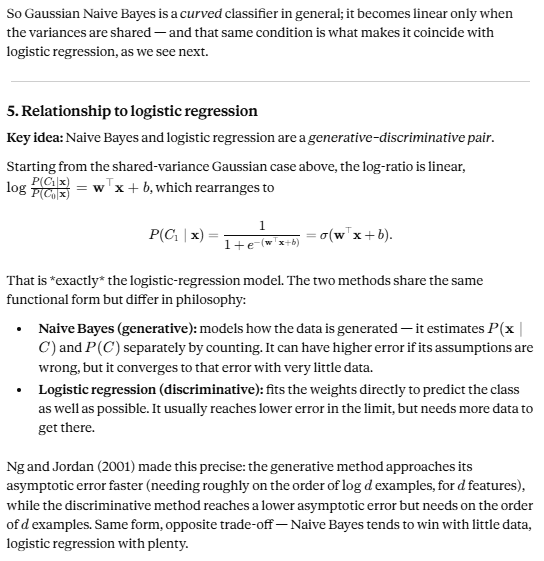
Naïve Bayes is a simple yet powerful probabilistic classifier built on Bayes’ theorem, widely used for its speed, interpretability, and surprisingly strong performance despite its “naïve” assumption that features are conditionally independent given the class. When a feature is continuous — like age or income — the Gaussian variant estimates its likelihood using the normal distribution, fitting a separate mean and standard deviation for each class. This tutorial walks through the complete theory, a fully verified worked numerical example (cross-checked against scikit-learn), and the deeper concepts most often probed in machine learning interviews — from numerical stability tricks to its exact relationship with Logistic Regression and Linear Discriminant Analysis.
The full tutorial — with every calculation shown step by step — is available in the PDF below.
Logistic Regression
Logistic regression is the standard model for predicting a binary outcome — Yes/No, 0/1 — such as whether a customer will buy, a loan will default, or a patient will respond to treatment. Unlike linear regression, it doesn’t predict the outcome directly; it predicts the probability of the outcome by passing a linear score through the sigmoid function, keeping every prediction safely between 0 and 1. Its coefficients are estimated using Maximum Likelihood Estimation, and are interpreted through odds ratios rather than raw units, making the model both accurate and genuinely explainable. This makes logistic regression the default baseline for binary classification and propensity modelling across marketing, healthcare, and finance.
Bayesian Belief Networks
A Bayesian belief network is a compact, graph-based way to represent a joint probability distribution over many random variables. It combines a directed acyclic graph (DAG) — where nodes are variables and edges capture direct probabilistic influence — with a set of local conditional probability distributions (CPDs). Representing a joint distribution explicitly needs an exponential number of parameters (2ⁿ−1 for n binary variables), which is computationally, cognitively, and statistically infeasible beyond a handful of variables. Bayesian networks solve this by exploiting conditional independence: each variable depends directly only on its parents in the graph, letting the full distribution factorize into small local pieces via the chain rule for Bayesian networks — often shrinking the parameter count from exponential to linear.
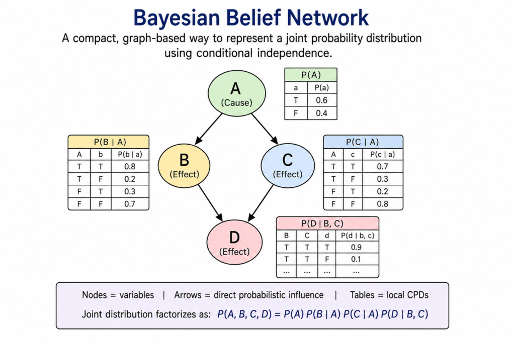
The graph carries a precise dual meaning: it is simultaneously a scaffold for factorizing a distribution and a compact encoding of independence assumptions, readable directly off the structure through d-separation. This structure supports natural human reasoning patterns — causal reasoning (cause → effect), evidential reasoning (effect → cause), and intercausal reasoning, or “explaining away,” where evidence for one cause lowers belief in a rival cause. The Naïve Bayes classifier is the simplest special case, with one class node and conditionally independent features. Bayesian networks have driven real applications in genetics, medical diagnosis, and decision support — and remain a foundational tool in modern probabilistic and causal reasoning.
The complete tutorial — with worked numerical examples, d-separation, and the theory of I-maps and I-equivalence — is available in the PDF below.
Key Conceptual Challenges in Bayesian Networks
1. Exponential Representation → Compact Factorization
A joint distribution over n binary variables needs 2ⁿ−1 parameters — exponential. A Bayesian network avoids this using a DAG plus conditional-independence assumptions, factorizing:
P(X₁,X₂,X₃,X₄) = P(X₁)P(X₂|X₁)P(X₃|X₁)P(X₄|X₂,X₃)
Key distinction: the chain rule is always valid and gives no compression by itself — compression comes strictly from the conditional-independence structure the graph encodes on top of it. Chain rule = identity; Bayesian-network factorization = chain rule + independence structure.
2. Conditional Independence and d-Separation
(X ⊥ Y | Z) means P(X|Y,Z) = P(X|Z). These independencies are not read off single arrows — they follow from the whole graph via d-separation, through three basic patterns:
- X→Z→Y: conditioning on Z blocks the path.
- X→Z←Y (v-structure): X, Y independent until Z is observed — conditioning creates dependence (explaining away).
- X←Z→Y: Z is a common cause; conditioning on Z blocks the association.
Chain: DAG structure → d-separation → conditional independencies → factorization → inference.
3. Reasoning Types, and the Causality Trap
P(X₁,…,Xₙ) = ∏ᵢ P(Xᵢ|Pa(Xᵢ)) supports causal reasoning (cause→effect), evidential reasoning (effect→cause), and intercausal reasoning / explaining away (one cause’s evidence shifts belief in a rival cause).
Critical distinction: a DAG is fundamentally a probabilistic model — it encodes statistical dependencies, not automatically causal mechanisms. Causal interpretation requires assumptions beyond the graph itself.
4. The Markov Blanket
Parents and children alone do not shield a node from the rest of the network — explaining away means co-parents matter too:
MB(X) = Parents(X) ∪ Children(X) ∪ CoParents(X)
Given MB(X), X is independent of everything else. This underlies Gibbs sampling and local structure learning. A candidate who forgets co-parents hasn’t internalized d-separation.
5. Why Observational Data Can’t Fix Causal Direction
I-equivalent DAGs (same skeleton, same immoralities) encode identical independencies — no statistical test distinguishes X→Y from Y→X within an equivalence class. This is why structure learning outputs a CPDAG, not a single DAG. Recovering true direction needs interventional data or assumptions outside the graph — the exact boundary between a statistical DAG and a causal diagram.
6. NP-Hardness and Treewidth
Exact inference is NP-hard in general; Variable Elimination’s cost is exponential in the induced width of the elimination order — not the variable count directly. A tree-structured network (width 1) is linear-time exact; a dense network can be intractable regardless of ordering, since finding the optimal order is itself NP-hard. The bottleneck is structural (treewidth), not size — this is why approximate inference (loopy BP, sampling) exists.
Neural Networks
Introduction to Neural Networks
This tutorial traces the earliest neural network models through one unifying idea — the straight-line decision boundary. A single neuron computes a weighted sum and fires on one side of the line b + Σwᵢxᵢ = 0, so it can only solve problems that are linearly separable (like AND and OR); XOR is not, and no single unit can learn it. Around this idea the models differ only in how the line is found: the McCulloch–Pitts neuron fixes its weights and threshold by hand with no learning at all; the Hebb net sets them in a single correlational pass (“fire together, wire together”); the perceptron learns by error correction, updating weights only when it misclassifies and converging whenever a separating line exists; and the ADALINE learns by least-squares, using the delta rule (Widrow–Hoff / LMS) to minimise squared error via gradient descent. When one line is not enough, MADALINE stacks two trainable ADALINEs under a fixed OR unit to combine lines and finally solve XOR. Read end to end, it shows the progression from hand-set to trained neurons and sets up the perceptron and the multilayer nets that follow. Download the below file for more detail.
The Perceptron
The perceptron, introduced by Rosenblatt in 1958, is the first neural network that learns its decision line by correcting its own mistakes. Like the earlier models it computes a weighted sum y_in = b + Σwᵢxᵢ and fires on one side of the boundary b + Σwᵢxᵢ = 0, but instead of fixing the weights by hand or in a single pass, it trains iteratively: for each pattern it compares its output with the target, and only when it misclassifies does it nudge the weights and bias by wᵢ += α·t·xᵢ and b += α·t. Correctly classified patterns cause no change, so learning slows as the net improves. Its great guarantee is the perceptron convergence theorem: if the data are linearly separable, the rule is certain to find a separating line in a finite number of steps — though it settles for any correct boundary, not the best-placed one. That same strength is its limit: on non-separable problems such as XOR it never settles, because no single line exists. The perceptron therefore marks the true beginning of trainable neural networks, bridging the hand-set neurons before it and the error-driven, multilayer networks — trained by the delta rule and backpropagation — that follow.
Backpropagation
Backpropagation is the reverse-mode automatic-differentiation algorithm that efficiently computes the gradient of a scalar loss (cost) function with respect to every weight and bias by recursively applying the chain rule across the computational graph. After the forward pass yields each neuron’s pre-activation (net = Σwx + b), activation (out = σ(net)), and the final loss, the backward pass propagates the error signal from output to input, computing at each node a local gradient or delta (∂E/∂net) , the product of the incoming upstream gradient and the activation’s derivative, e.g. o(1−o) for sigmoid — so every weight gradient equals delta × input. These gradients drive gradient-descent optimizers (batch, stochastic, mini-batch SGD, Momentum, RMSProp, Adam), scaled by the learning rate η, updating parameters as w_new = w_old − η ∂E/∂w over successive epochs. Key interview terms include partial derivatives, the Jacobian, credit assignment, and the vanishing/exploding-gradient problem ,caused by repeatedly multiplying small or large derivatives (sigmoid saturation, dead ReLUs) – mitigated by ReLU/tanh activations, Xavier/He initialization, batch normalization, residual connections, and gradient clipping. Overfitting is curbed by regularization (L2/weight decay, dropout), while vectorization and GPU parallelism give speed. For recurrent networks it generalizes to backpropagation-through-time (BPTT). Fundamentally, backpropagation is not a collection of formulas but a single idea : the chain rule applied backward : enabling scalable, end-to-end gradient-based training in modern deep-learning frameworks
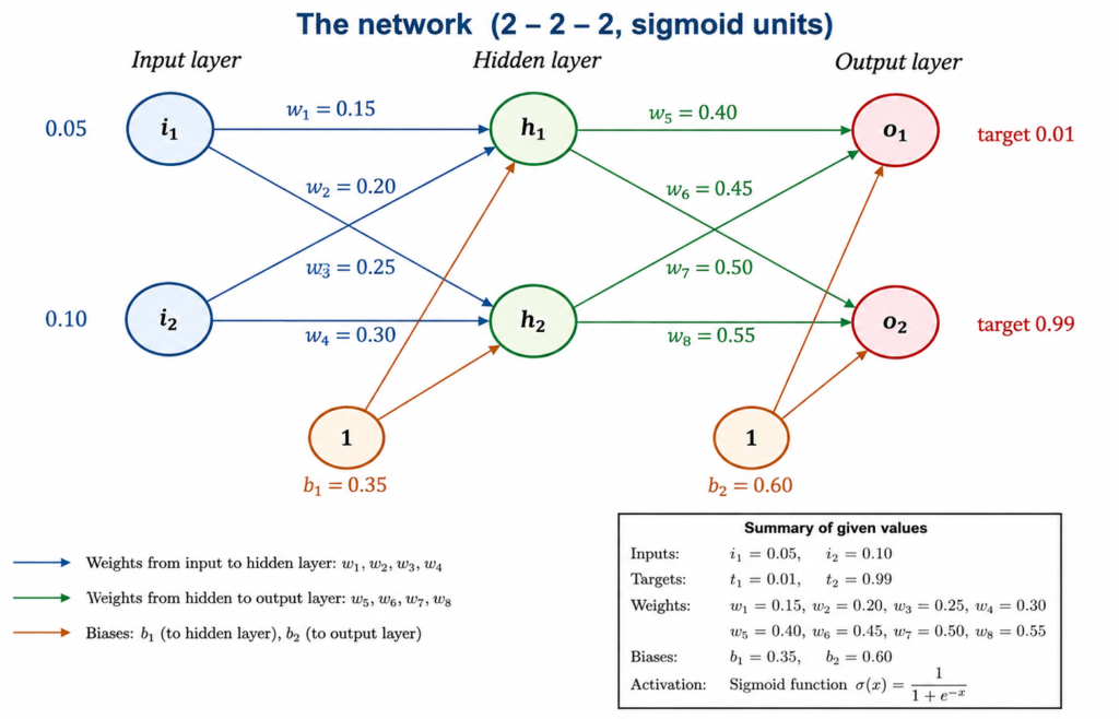
Please see the attached solution for complete backpropagation below.
Ensembles: The Bias–Variance Tradeoff
Every predictive model’s error can be broken down into three fundamental sources: irreducible noise inherent to the data, bias from a model too simple to capture the true pattern, and variance from a model too sensitive to the particular training sample it happened to see. This decomposition — Error = Noise + Bias² + Variance — is the theoretical backbone behind why ensemble methods work at all, and why two seemingly similar techniques, bagging and boosting, actually attack completely different halves of this equation. Bagging trains many strong, independent models on bootstrap resamples of the data and averages their predictions, directly shrinking variance — its effectiveness depends critically on how correlated the individual models are, which is precisely why Random Forest deliberately decorrelates its trees to outperform plain bagging. Boosting instead trains many weak models sequentially, each correcting the errors of the last, directly shrinking bias — with a rigorous guarantee that training error decays exponentially fast, provided each weak learner clears even a small edge over random guessing. Understanding this tradeoff is essential to knowing which ensemble technique to reach for, and why.
- Every model’s error splits exactly into Irreducible Noise + Bias² + Variance
- Bagging reduces variance by averaging independent, strong models
- Boosting reduces bias by sequentially combining weak learners
- Random Forest works by deliberately decorrelating trees, not just bagging them
- AdaBoost’s training error provably shrinks exponentially fast with more rounds
The complete tutorial — with the full derivation, verified formulas, and a worked numerical example — is available in the PDF below.
Ensemble learning
Ensemble learning is a machine-learning paradigm that combines many base learners into one stronger predictor, exploiting the bias–variance trade-off: a model’s expected squared error decomposes exactly into bias² (error from oversimplified assumptions, causing underfitting), variance (sensitivity to the training set, causing overfitting), and irreducible noise σ². Ensembles work because averaging M diverse models with pairwise correlation ρ reduces variance as ρσ² + (1−ρ)σ²/M — so both more models and less-correlated (decorrelated) models help. Bagging (Bootstrap Aggregating) trains independent, parallel models on bootstrap samples drawn with replacement (leaving ≈36.8% out-of-bag tuples for free validation, since (1−1/N)^N→1/e) and combines them by majority vote or averaging; it mainly reduces variance, making it ideal for low-bias, high-variance learners like deep decision trees. Random Forests extend bagging by sampling a random feature subset (≈√p) at each split, further decorrelating the trees. Boosting instead builds models sequentially, each re-weighting the tuples the previous one misclassified so later learners focus on hard cases; AdaBoost computes a weighted error, a classifier weight α = ln((1−error)/error), updates tuple weights (with normalization), and predicts by weighted vote, converting weak learners into a strong one by reducing bias. Gradient Boosting (XGBoost, LightGBM) generalizes this by fitting each model to the residual gradient of a differentiable loss. Fundamentally: bagging averages away variance; boosting chips away bias.
Expectation–Maximization (EM) algorithm
The Expectation–Maximization (EM) algorithm is an iterative method for finding maximum-likelihood estimates of model parameters when the data depend on hidden (latent) variables that are never observed, such as which coin produced each set of tosses. It starts from an initial guess of the parameters and repeats two steps. In the E-step (Expectation), it uses the current parameters to compute the probability of each possible value of the hidden variable for every observation (the “responsibilities”), and from these it forms expected counts or statistics. In the M-step (Maximization), it re-estimates the parameters by maximizing the likelihood using those expected counts, as if they were real data. Each iteration is guaranteed never to decrease the likelihood, and the process stops when the parameter change falls below a small threshold ε. EM converges to a local maximum, so the final result can depend on the starting values. It is widely used in Gaussian mixture models, hidden Markov models (Baum–Welch), clustering, and handling missing data.
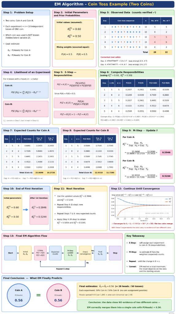
Step 6: Compute Responsibilities (using θ_A⁽⁰⁾ = 0.60, θ_B⁽⁰⁾ = 0.50)
Experiment 1: x = 5 heads, n − x = 5 tails, n = 10
(a) Binomial coefficient
C(10, 5) = 10! / (5! × 5!) = 252
(b) Likelihood under Coin A: P(E|A)
P(E|A) = C(10, 5) × θ_A⁵ × (1 − θ_A)⁵
= 252 × 0.6⁵ × 0.4⁵
= 252 × 0.07776 × 0.01024
= 252 × 0.0007962624
= 0.2006581 ≈ 0.2007
(c) Likelihood under Coin B: P(E|B)
P(E|B) = C(10, 5) × θ_B⁵ × (1 − θ_B)⁵
= 252 × 0.5⁵ × 0.5⁵
= 252 × 0.5¹⁰
= 252 / 1024
= 0.2460938 ≈ 0.2461
(d) Responsibility of Coin A: P(Z=A|E)
Bayes’ rule gives:
P(Z=A|E) = P(E|A)·P(A) / [P(E|A)·P(A) + P(E|B)·P(B)]
Since P(A) = P(B) = 0.5, the priors cancel:
P(Z=A|E) = 0.2006581 / (0.2006581 + 0.2460938)
= 0.2006581 / 0.4467519
= 0.449149 ≈ 0.4491
(e) Responsibility of Coin B: P(Z=B|E)
P(Z=B|E) = 1 − P(Z=A|E)
= 1 − 0.4491
= 0.5509
Interpretation: there is a 44.91% chance Experiment 1 was produced by Coin A and a 55.09% chance it was produced by Coin B.
Step 7: Expected Counts for Coin A
Experiment 1: x = 5, n − x = 5, P(Z=A|E) = 0.4491 (from Step 6)
Each head and tail is credited to Coin A in proportion to Coin A’s responsibility.
Expected heads for Coin A
Exp. H for A = P(Z=A|E) × x
= 0.4491 × 5
= 2.2455
Expected tails for Coin A
Exp. T for A = P(Z=A|E) × (n − x)
= 0.4491 × 5
= 2.2455
Interpretation: of the 5 heads and 5 tails in Experiment 1, about 2.2455 heads and 2.2455 tails are credited to Coin A.
Step 8: Expected Counts for Coin B
Experiment 1: x = 5, n − x = 5, P(Z=B|E) = 0.5509 (from Step 6)
Expected heads for Coin B
Exp. H for B = P(Z=B|E) × x
= 0.5509 × 5
= 2.7545
Expected tails for Coin B
Exp. T for B = P(Z=B|E) × (n − x)
= 0.5509 × 5
= 2.7545
Check: the counts credited to A and B must add back to the observed counts.
- Heads: 2.2455 (A) + 2.7545 (B) = 5 ✔
- Tails: 2.2455 (A) + 2.7545 (B) = 5 ✔
Interpretation: the remaining 2.7545 heads and 2.7545 tails of Experiment 1 are credited to Coin B
K-means clustering
See below link for K_Means & K-Modes
K-Medoids
K-Medoids is a partitioning-based clustering algorithm in which the center of each cluster is an actual data point from the dataset, called a medoid. Unlike K-Means, where the cluster center is a calculated centroid that may not correspond to an existing observation, K-Medoids selects representative data points and assigns other points to the nearest medoid based on a chosen dissimilarity measure. The attached tutorial presents K-Medoids using a small dataset of 10 points and two clusters, with Manhattan distance used for calculating dissimilarity. It explains the complete procedure step by step, beginning with the selection of two initial medoids, followed by distance calculation and assignment of each non-medoid point to its nearest medoid. The tutorial then calculates the initial total cost by summing the minimum distances of the points to their assigned medoids. A medoid–non-medoid swap is subsequently proposed, after which all distances, cluster assignments, and the new total cost are recalculated. The example shows an initial cost of 20 and a new cost of 22, producing a swap cost of +2; therefore, the proposed swap is rejected and the original medoids are retained. The tutorial also compares K-Means and K-Medoids, highlights their differences, summarizes the three important formulas—Manhattan distance, total cost, and swap cost—and provides an exam-friendly sequence for remembering the complete K-Medoids procedure. It concludes with an important clarification that rejecting one swap does not by itself establish global optimality; full convergence requires evaluating relevant possible swaps until no further improvement is obtained.
Summary
- Actual data points are used as medoids.
- Uses distance-based cluster assignment.
- Demonstrates Manhattan distance calculation.
- Swap cost determines whether a medoid swap is accepted.
- Procedure continues until no further improvement.
DBSCAN
DBSCAN (Density-Based Spatial Clustering of Applications with Noise) is a density-based clustering algorithm that forms clusters by identifying regions containing sufficiently dense groups of points while treating isolated observations as noise. Unlike K-Means, DBSCAN does not require the number of clusters to be specified in advance. The algorithm uses two key parameters: ε (epsilon), which defines the maximum distance for two points to be considered neighbors, and MinPts, which specifies the minimum number of points required within an ε-neighborhood for a point to be classified as a core point. The attached tutorial explains the complete DBSCAN procedure using a distance matrix with ε = 1.9 and MinPts = 4. It introduces the three types of DBSCAN points—core, border, and noise—and demonstrates how ε-neighborhoods are calculated and used to classify every point. The tutorial then explains density connectivity and shows how core points expand into clusters through density-connected points rather than simple geometric proximity. For the given dataset, the final result contains two clusters and one noise point: Cluster 1 = {P1, P2, P3, P10, P11, P12}, Cluster 2 = {P4, P5, P6, P7, P8}, and Noise = {P9}. It also discusses important practical considerations, including the effects of selecting ε too small or too large, increasing MinPts, feature scaling, distance-metric selection, high-dimensional data, anomaly detection, and datasets with different densities. The tutorial emphasizes that DBSCAN can discover non-spherical clusters and that cluster membership depends on density connectivity rather than ordinary pairwise closeness.
Summary
- Density-based clustering that does not require the number of clusters.
- Uses ε and MinPts to identify dense regions.
- Classifies points as core, border, or noise.
- Forms clusters through density connectivity.
- Can detect arbitrarily shaped clusters and noise.