Hypothesis Space

Source: Tom M. Mitchell, Machine Learning (1997), Concept Learning and the General-to-Specific Ordering

The Big Idea in One Minute

Suppose your friend Aldo enjoys his favourite water sport on some days and not on others. You watch a few days, note the weather, and note whether Aldo enjoyed the sport. Now you want a rule that predicts, for any new day, whether Aldo will enjoy the sport.

Mitchell calls this concept learning: inferring a boolean-valued function from training examples of its input and output. “Boolean-valued” simply means the answer is Yes (1) or No (0).

Key insight: Before learning starts, we must decide what kinds of rules the learner is even allowed to consider. The set of ALL rules the learner is allowed to consider is called the hypothesis space, H. Learning = searching inside H for the rule that best fits the training data.

The EnjoySport Task

Each day is described by six attributes. These attributes and their possible values:

Attribute	Possible values	How many values?
Sky	Sunny, Cloudy, Rainy	3
AirTemp	Warm, Cold	2
Humidity	Normal, High	2
Wind	Strong, Weak	2
Water	Warm, Cool	2
Forecast	Same, Change	2

The training examples. Each row is one observed day; the last column is the answer we want to learn to predict:

Example	Sky	AirTemp	Humidity	Wind	Water	Forecast	EnjoySport
1	Sunny	Warm	Normal	Strong	Warm	Same	Yes
2	Sunny	Warm	High	Strong	Warm	Same	Yes
3	Rainy	Cold	High	Strong	Warm	Change	No
4	Sunny	Warm	High	Strong	Cool	Change	Yes

What Exactly Is a “Hypothesis” Here?

A hypothesis is one candidate rule. Every hypothesis is a vector of six constraints — one constraint for each attribute (Sky, AirTemp, Humidity, Wind, Water, Forecast). For each attribute, the constraint can be exactly one of three things:

• “?” — any value is acceptable for this attribute (“don’t care”).
• A specific value (e.g., Warm) — this exact value is required.
• “Ø” — no value is acceptable (the empty constraint).

A hypothesis h classifies a day x as positive (h(x) = 1, i.e., “Aldo enjoys sport”) if and only if the day satisfies all six constraints. Otherwise it classifies the day as negative (h(x) = 0).

Three example hypotheses (read them like sentences):

Hypothesis	Plain-language meaning
⟨?, Cold, High, ?, ?, ?⟩	“Aldo enjoys sport on any cold day with high humidity, regardless of everything else.”
⟨?, ?, ?, ?, ?, ?⟩	The most general hypothesis: every day is positive. “Aldo enjoys sport every day.”
⟨Ø, Ø, Ø, Ø, Ø, Ø⟩	The most specific hypothesis: no day is positive. “Aldo never enjoys sport.” (One single Ø anywhere is already enough for this.)

Common student mistake: “?” and “Ø” are opposites. “?” says “everything passes here”; “Ø” says “nothing passes here.” Because a day must satisfy ALL six constraints, even one Ø makes the whole hypothesis reject every day.

The Standard Notation (Learn These Five Symbols)

Symbol	Name	Meaning in EnjoySport
X	Instance space	The set of ALL possible days (every combination of the six attribute values).
c	Target concept	The true, unknown function we want. c : X → {0, 1}. Here c(x) = 1 if EnjoySport = Yes, c(x) = 0 if No.
D	Training examples	The observed pairs ⟨x, c(x)⟩ — the four rows of the table above.
H	Hypothesis space	The set of ALL hypotheses the learner may consider. Determined by the human designer’s choice of representation (here: conjunctions of six constraints).
h	One hypothesis	One member of H. Each h : X → {0, 1}. The goal: find h such that h(x) = c(x) for all x in X.

The Inductive Learning Hypothesis: any hypothesis that approximates the target function well over a sufficiently large set of training examples will also approximate it well over unobserved examples. This is an ASSUMPTION, not a theorem — the learner only ever sees the training data, so this assumption is the only justification for generalizing beyond it.

Concept Learning = Searching the Hypothesis Space

Concept learning is the task of searching through a large space of hypotheses implicitly defined by the hypothesis representation, to find the hypothesis that best fits the training examples. The EnjoySport space is small and finite; most practical tasks have enormous or infinite hypothesis spaces, so we need clever search — which is where the general-to-specific ordering and FIND-S come in.

Very simple explanation: Imagine you are trying to guess a secret rule. You have some examples:

Weather	Wind	Play Tennis?
Sunny	Weak	Yes
Rainy	Strong	No
Cloudy	Weak	Yes

Your job is to discover the hidden rule. You may think of many possible rules: Rule 1: Always play. Rule 2: Play only when sunny. Rule 3: Play when wind is weak. Rule 4: Play when not rainy. Rule 5: Play when sunny and wind is weak. Each possible rule is called a hypothesis. So, concept learning = searching through many possible rules to find the best one. A hypothesis space is simply the collection of all possible rules (hypotheses) that the algorithm can consider — think of it as a library of possible answers. The algorithm searches this library to find the best rule.

How Big Is the EnjoySport Hypothesis Space?

Step 1 — size of the instance space X. Multiply the number of values of each attribute:

|X| = 3 × 2 × 2 × 2 × 2 × 2 = 96 possible distinct days.

Step 2 — syntactically distinct hypotheses. For each attribute, the constraint slot can be filled with any of its values, PLUS “?”, PLUS “Ø”. So Sky has 3 + 2 = 5 choices, and each of the other five attributes has 2 + 2 = 4 choices:

5 × 4 × 4 × 4 × 4 × 4 = 5120 syntactically distinct hypotheses.

Step 3 — semantically distinct hypotheses. Every hypothesis containing one or more Ø classifies EVERY day as negative — so all of them mean the same thing. Count them as ONE hypothesis, and count the Ø-free hypotheses separately. A Ø-free hypothesis has (values + 1 for “?”) choices per attribute: 4 for Sky, 3 for each other attribute:

1 + (4 × 3 × 3 × 3 × 3 × 3) = 1 + 972 = 973 semantically distinct hypotheses.

Memory hook: Instances: multiply the values (96). Syntactic: values + 2 per slot (5120). Semantic: values + 1 per slot, then add 1 for the single all-negative hypothesis (973).

An honest limitation: H contains only conjunctions (AND-rules). A concept like “Sky = Sunny OR Sky = Cloudy” is not expressible in this H at all. Choosing H fixes, in advance, what the learner can and cannot ever learn.

The General-to-Specific Ordering (The Structure Inside H)

H is not just a bag of 973 rules — it has a natural structure. Consider two hypotheses:

h₁ = ⟨Sunny, ?, ?, Strong, ?, ?⟩ h₂ = ⟨Sunny, ?, ?, ?, ?, ?⟩

h₂ imposes fewer constraints, so it classifies more days as positive. In fact every day classified positive by h₁ is also classified positive by h₂. So we say h₂ is more general than h₁.

Formal definition: hⱼ is more_general_than_or_equal_to hₖ (written hⱼ ≥g hₖ) if and only if every instance that satisfies hₖ also satisfies hⱼ.

• With h₃ = ⟨Sunny, ?, ?, ?, Cool, ?⟩: h₂ is more general than h₃ as well. But h₁ and h₃ are not comparable — neither is more general than the other (their positive sets overlap but neither contains the other).
• So ≥g is a partial order on H (reflexive, antisymmetric, transitive) — partial, not total, because some pairs are simply incomparable.
• Important: the ordering depends only on which instances satisfy the hypotheses. It is independent of the target concept and of the training data.

Why care? Because this structure lets algorithms search even huge hypothesis spaces without enumerating every hypothesis. FIND-S is the first such algorithm: start at the most specific hypothesis ⟨Ø,Ø,Ø,Ø,Ø,Ø⟩ and generalize it minimally each time it fails to cover a positive training example.

Worked Numerical Exercise

Problem. A learner must predict whether a fruit is “Tasty” (Yes/No). Each fruit is described by three attributes: Colour (Red, Green, Yellow), Size (Big, Small), Shape (Round, Long). Hypotheses are conjunctions of constraints using specific values, “?”, and “Ø”, exactly as in EnjoySport. Compute: (a) the size of the instance space, (b) the number of syntactically distinct hypotheses, (c) the number of semantically distinct hypotheses.

Solution

(a) Instance space |X|. Each fruit is one combination of attribute values. Colour has 3 values, Size has 2, Shape has 2:

|X| = 3 × 2 × 2 = 12 possible distinct fruits.

(b) Syntactically distinct hypotheses. Each attribute slot can hold: one of its specific values, or “?”, or “Ø”. So the number of choices per slot is (number of values + 2): Colour 3+2 = 5, Size 2+2 = 4, Shape 2+2 = 4:

5 × 4 × 4 = 80 syntactically distinct hypotheses.

(c) Semantically distinct hypotheses. Any hypothesis with at least one Ø classifies every fruit negative — all such hypotheses are one and the same rule (“nothing is tasty”). Count that as 1. The remaining hypotheses have no Ø, so each slot has (values + 1) choices: Colour 3+1 = 4, Size 2+1 = 3, Shape 2+1 = 3:

1 + (4 × 3 × 3) = 1 + 36 = 37 semantically distinct hypotheses.

Sanity check: 80 syntactic − 36 Ø-free = 44 hypotheses contain a Ø; all 44 collapse into the single all-negative rule; 36 + 1 = 37. Consistent. ✓

Summary

The hypothesis space H is the complete menu of rules a learner is permitted to consider, and it is fixed in advance by the human’s choice of representation. In EnjoySport, H = all conjunctions of six constraints (value / ? / Ø), giving 5120 syntactic and 973 semantic hypotheses over an instance space of only 96 days. Learning is search through H for an h with h(x) = c(x); the inductive learning hypothesis is the assumption that fitting the training data well means fitting unseen data well; and the general-to-specific partial ordering ≥g is the structure that makes efficient search (FIND-S and beyond) possible.

Same treatment as Hypothesis Space — here’s the paste-ready FIND-S content, MCQs and practice exercises removed, worked solved exercise kept:

---

The FIND-S Algorithm

Finding a Maximally Specific Hypothesis. Source: Tom M. Mitchell, Machine Learning (1997)

The Big Idea in One Minute

We know from the previous section that learning = searching the hypothesis space H. But H can be huge. How do we search it without checking every hypothesis one by one?

Mitchell’s answer: use the more_general_than partial ordering as a ladder. FIND-S starts at the very bottom of the ladder (the most specific hypothesis possible) and climbs upward — generalizing — only when a positive training example forces it to. It never generalizes more than necessary, and it completely ignores negative examples.

FIND-S in one sentence: Begin with the most specific hypothesis in H, and each time it fails to cover an observed positive example, generalize it just enough (“minimally”) to cover that example. (We say a hypothesis “covers” a positive example if it correctly classifies the example as positive.)

The Algorithm

FIND-S Algorithm

1. Initialize h to the most specific hypothesis in H
2. For each positive training instance x:
   • For each attribute constraint aᵢ in h: if the constraint aᵢ is satisfied by x, then do nothing; else replace aᵢ in h by the next more general constraint that is satisfied by x
3. Output hypothesis h

“Next more general constraint” in this representation means exactly two possible moves per slot:

• Ø → the specific value seen in the example (e.g., Ø becomes Sunny). This is the smallest possible generalization from Ø.
• A specific value → ? (e.g., Normal becomes ?). If the stored value disagrees with the example’s value, the only constraint general enough to accept both is “?”.

Two things students always miss: (1) FIND-S looks only at POSITIVE examples — negative examples are simply skipped. (2) Once a slot becomes “?”, it can never go back; generalization is one-way, upward.

The Training Data

Example	Sky	AirTemp	Humidity	Wind	Water	Forecast	EnjoySport
1	Sunny	Warm	Normal	Strong	Warm	Same	Yes
2	Sunny	Warm	High	Strong	Warm	Same	Yes
3	Rainy	Cold	High	Strong	Warm	Change	No
4	Sunny	Warm	High	Strong	Cool	Change	Yes

Full Trace of FIND-S (Every Step Explained)

Step 0 — Initialization

h₀ = ⟨Ø, Ø, Ø, Ø, Ø, Ø⟩

This hypothesis says “no day is positive.” It is the most specific member of H — the bottom of the ladder.

Step 1 — Example 1: ⟨Sunny, Warm, Normal, Strong, Warm, Same⟩, Yes (positive)

Is Example 1 covered by h₀? No — none of the Ø constraints is satisfied by this example. So each Ø is replaced by the next more general constraint that fits the example: the attribute value itself.

h₁ = ⟨Sunny, Warm, Normal, Strong, Warm, Same⟩

h is still very specific: it asserts that ALL days are negative except the one exact day we observed.

Step 2 — Example 2: ⟨Sunny, Warm, High, Strong, Warm, Same⟩, Yes (positive)

Compare slot by slot with h₁. Sky: Sunny = Sunny ✓ keep. AirTemp: Warm = Warm ✓ keep. Humidity: h says Normal, example says High ✗ — disagreement → replace with “?”. Wind, Water, Forecast: all agree ✓ keep.

h₂ = ⟨Sunny, Warm, ?, Strong, Warm, Same⟩

Step 3 — Example 3: ⟨Rainy, Cold, High, Strong, Warm, Change⟩, No (negative)

FIND-S IGNORES it. h₃ = h₂, unchanged.

Why is ignoring negative examples justified? Mitchell’s argument: we assume the target concept c is in H and is consistent with the positive training examples. Then c must be more_general_than_or_equal_to the current h (h is the most specific hypothesis fitting the positives). Since c never covers a negative example, and h is contained within c, h can never cover a negative example either — so no revision is ever needed in response to a negative example. Verify it here: h₂ requires Sky = Sunny, but Example 3 has Sky = Rainy, so h₂ already correctly classifies Example 3 as negative.

Step 4 — Example 4: ⟨Sunny, Warm, High, Strong, Cool, Change⟩, Yes (positive)

Compare with h₂ slot by slot. Sky: Sunny ✓. AirTemp: Warm ✓. Humidity: already “?” ✓. Wind: Strong ✓. Water: h says Warm, example says Cool ✗ → “?”. Forecast: h says Same, example says Change ✗ → “?”.

h₄ = ⟨Sunny, Warm, ?, Strong, ?, ?⟩ ← FINAL OUTPUT

Read it as a sentence: “Aldo enjoys his sport on sunny, warm, strong-wind days — humidity, water temperature and forecast do not matter.”

The whole trace in one summary table:

After seeing…	Type	Hypothesis h	What changed
(start)	—	⟨Ø, Ø, Ø, Ø, Ø, Ø⟩	Initialized to most specific
Example 1	+	⟨Sunny, Warm, Normal, Strong, Warm, Same⟩	All six Ø → the observed values
Example 2	+	⟨Sunny, Warm, ?, Strong, Warm, Same⟩	Humidity → ?
Example 3	−	⟨Sunny, Warm, ?, Strong, Warm, Same⟩	Nothing — negative examples ignored
Example 4	+	⟨Sunny, Warm, ?, Strong, ?, ?⟩	Water → ?, Forecast → ?

Picture in your head: the search moves from hypothesis to hypothesis, from the most specific end toward more general hypotheses, along ONE chain of the partial ordering. At each step h is generalized only as far as necessary to cover the new positive example. Hence, at every stage, h is the MOST SPECIFIC hypothesis consistent with the training examples seen so far — that is why the algorithm is called FIND-S (S = specific).

What FIND-S Guarantees — and Its Four Honest Problems

Guarantee: for hypothesis spaces described by conjunctions of attribute constraints (like EnjoySport’s H), FIND-S is guaranteed to output the most specific hypothesis in H consistent with the positive training examples. Its final hypothesis will also be consistent with the negative examples PROVIDED (i) the correct target concept is contained in H, and (ii) the training examples are correct (no noise). Both provisos matter — drop either one and the guarantee collapses.

The questions FIND-S leaves unanswered — the standard exam questions on this topic:

1. Has the learner converged to the correct target concept? FIND-S finds A hypothesis consistent with the data, but it cannot tell whether it is the ONLY consistent one in H, or one among many. It cannot even characterize its own uncertainty.
2. Why prefer the most specific hypothesis? If several hypotheses are consistent with the data, it is unclear why we should prefer the most specific one over the most general one, or something in between.
3. Are the training examples consistent (noise-free)? Real data contains errors. Noisy examples can severely mislead FIND-S, precisely because it ignores negative examples — it has no way to even detect an inconsistency.
4. What if there are several maximally specific consistent hypotheses? In EnjoySport’s H there is always a unique most specific consistent hypothesis, but for other hypothesis spaces there can be several — and FIND-S has no policy for that situation.

These four weaknesses are exactly the motivation for the Candidate Elimination Algorithm, which comes next.

Worked Numerical Exercise (Fully Solved, Step by Step)

Problem. A college wants to learn the concept “Student gets placed” (Yes/No). Attributes: CGPA (High, Low), Communication (Good, Poor), Internship (Yes, No), Backlogs (None, Some). Run FIND-S on the following four training examples, showing the hypothesis after every example.

Example	CGPA	Communication	Internship	Backlogs	Placed
1	High	Good	Yes	None	Yes
2	High	Good	No	None	Yes
3	Low	Poor	No	Some	No
4	High	Good	No	Some	Yes

Solution

Step 0. h₀ = ⟨Ø, Ø, Ø, Ø⟩ (most specific; classifies every student as not placed).

Step 1 — Example 1 (positive). h₀ covers nothing, so every Ø is replaced by the example’s value: h₁ = ⟨High, Good, Yes, None⟩.

Step 2 — Example 2 (positive). Compare slot by slot: CGPA High = High ✓; Communication Good = Good ✓; Internship: h says Yes, example says No ✗ → “?”; Backlogs None = None ✓. So h₂ = ⟨High, Good, ?, None⟩.

Step 3 — Example 3 (negative). Ignored. h₃ = h₂ = ⟨High, Good, ?, None⟩. (Check: h₂ requires CGPA = High; Example 3 has Low, so it is already correctly classified negative.)

Step 4 — Example 4 (positive). CGPA High ✓; Communication Good ✓; Internship already “?” ✓; Backlogs: h says None, example says Some ✗ → “?”.

FINAL: h₄ = ⟨High, Good, ?, ?⟩

In words: “A student is placed if CGPA is High and Communication is Good — internship and backlogs do not matter (according to this data).” Note honestly: this rule is only the most specific hypothesis consistent with these four examples; it is not guaranteed to be the true concept.

Summary

FIND-S searches the hypothesis space by climbing one chain of the general-to-specific ordering: start at ⟨Ø,…,Ø⟩, and for each positive example generalize each violated constraint minimally (Ø → value, value → ?), ignoring every negative example. On the EnjoySport data the trace is ⟨Ø,Ø,Ø,Ø,Ø,Ø⟩ → ⟨Sunny, Warm, Normal, Strong, Warm, Same⟩ → ⟨Sunny, Warm, ?, Strong, Warm, Same⟩ → (unchanged) → ⟨Sunny, Warm, ?, Strong, ?, ?⟩. It is guaranteed to output the most specific hypothesis consistent with the positive examples, and it is safe on negatives only if the target concept is in H and the data is noise-free. Its four weaknesses — no convergence test, no reason to prefer the most specific hypothesis, no tolerance or detection of noise, and no policy when several maximally specific hypotheses exist — motivate the Candidate Elimination Algorithm.

Candidate Elimination Algorithm

A Complete Worked Example on the EnjoySport Concept  

                                                                                                          @S S Roy

Introduction

The Candidate Elimination Algorithm (CEA) keeps track of all hypotheses consistent with the training data, not just one, by maintaining two boundaries: S (the most specific boundary) and G (the most general boundary).

Positive examples push S to become more general, and negative examples push G to become more specific, until the two boundaries close in on the version space — the set of every rule that fits the data.

The algorithm helps by showing every hypothesis still consistent with the data — so you know exactly how much uncertainty remains, and which next example would best narrow it down.

The Training Data (EnjoySport)

Example	Sky	AirTemp	Humidity	Wind	Water	Forecast	EnjoySport
1	Sunny	Warm	Normal	Strong	Warm	Same	Yes
2	Sunny	Warm	High	Strong	Warm	Same	Yes
3	Rainy	Cold	High	Strong	Warm	Change	No
4	Sunny	Warm	High	Strong	Cool	Change	Yes

Note: Example 3 is the only negative example (EnjoySport = No). All others are positive.

Initialization

The boundary sets are first initialized to the most specific and most general hypotheses possible:

S₀ = ⟨∅, ∅, ∅, ∅, ∅, ∅⟩        (most specific boundary)

G₀ = ⟨?, ?, ?, ?, ?, ?⟩        (most general boundary)

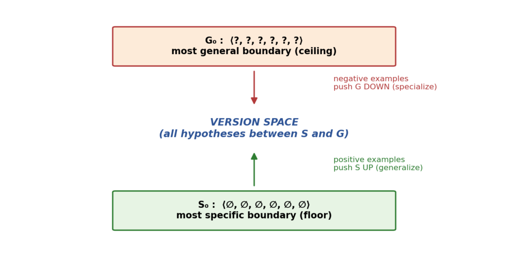
Figure 1: The two boundaries S and G, and the version space between them. Positive examples push S up; negative examples push G down.

The Algorithm

Initialize:  S ← most specific hypothesis ⟨∅, …, ∅⟩;  G ← most general hypothesis ⟨?, …, ?⟩

For each training example d:

If d is positive:

• Delete from G any rule inconsistent with d.

• Generalize S just enough to stay consistent with d.

If d is negative:

• Delete from S any rule inconsistent with d.

• Specialize G just enough to stay consistent with d.

Output: all rules consistent with the data (everything between S and G). If S = G, the exact concept has been found.

Remember: positives push S up (more general); negatives push G down (more specific).

Tracing the Algorithm Step by Step

Training Example 1 (Positive): ⟨Sunny, Warm, Normal, Strong, Warm, Same⟩ → Yes

When the first training example is presented, the algorithm checks the S boundary and finds that it is overly specific — it fails to cover this positive example. The boundary is therefore revised by moving it to the least more general hypothesis that covers the new example. There is no update to the G boundary, since G₀ already covers this example.

S₁ = { ⟨Sunny, Warm, Normal, Strong, Warm, Same⟩ }

G₁ = G₀ = ⟨?, ?, ?, ?, ?, ?⟩

Training Example 2 (Positive): ⟨Sunny, Warm, High, Strong, Warm, Same⟩ → Yes

The second training example (also positive) has a similar effect of generalizing S further to S₂. The Humidity values differ (Normal vs. High), so that position is generalized to “?”. G remains unchanged: G₂ = G₁ = G₀.

S₂ = { ⟨Sunny, Warm, ?, Strong, Warm, Same⟩ }

G₂ = G₁ = G₀ = ⟨?, ?, ?, ?, ?, ?⟩

Note: up to this point, the algorithm behaves exactly the same as FIND-S.

Important Observations Before Example 3

• Positive examples may force the S boundary of the version space to become increasingly general.

• Negative training examples play the complementary role of forcing the G boundary to become increasingly specific.

• The third example is negative, and it shows that G is currently too general.

• Being too general, G wrongly labels (incorrectly predicts) the new example as positive.

• So G must be tightened until it calls the example negative. Therefore, we are next going to see several alternative minimally more specific hypotheses.

Training Example 3 (Negative): ⟨Rainy, Cold, High, Strong, Warm, Change⟩ → No

The negative day is ⟨Rainy, Cold, High, Strong, Warm, Change⟩. The positive days so far are summarised by S₂ = ⟨Sunny, Warm, ?, Strong, Warm, Same⟩.

To specialize G₂ = ⟨?, ?, ?, ?, ?, ?⟩, we add one constraint at a time, using the value from the S-summary for that attribute (which guarantees the positive days still pass). Then we check whether it also rejects the negative day:

Add Constraint	Does it reject the negative day?	Kept?
Sky = Sunny	Yes — the negative day was Rainy	✓ Keep
AirTemp = Warm	Yes — the negative day was Cold	✓ Keep
Humidity = ?	No usable value — S₂ already has “?” for Humidity, so no constraint is available	✗ Out
Wind = Strong	No — the negative day also had Strong wind, so it is not rejected	✗ Out
Water = Warm	No — the negative day also had Warm water, so it is not rejected	✗ Out
Forecast = Same	Yes — the negative day was Change	✓ Keep

So, out of six attributes, only Sky, AirTemp, and Forecast give a constraint that the positive days satisfy but the negative day violates. All three become members of the new G₃ boundary set. Regarding S₃: the negative example does not touch S, so S₃ = S₂.

S₃ = S₂ = { ⟨Sunny, Warm, ?, Strong, Warm, Same⟩ }

G₃ = { ⟨Sunny, ?, ?, ?, ?, ?⟩,  ⟨?, Warm, ?, ?, ?, ?⟩,  ⟨?, ?, ?, ?, ?, Same⟩ }

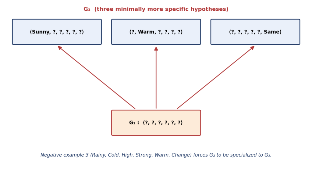
Figure 2: Negative example 3 forces G₂ to be specialized — all three minimally more specific hypotheses become members of the new G₃ boundary set.

Training Example 4 (Positive): ⟨Sunny, Warm, High, Strong, Cool, Change⟩ → Yes

This positive example generalizes S further: Water differs (Warm vs. Cool) and Forecast differs (Same vs. Change), so both positions become “?”.

It also affects G: the member ⟨?, ?, ?, ?, ?, Same⟩ is inconsistent with this positive example (its Forecast is Change), so that rule is deleted from G.

S₄ = { ⟨Sunny, Warm, ?, Strong, ?, ?⟩ }

G₄ = { ⟨Sunny, ?, ?, ?, ?, ?⟩,  ⟨?, Warm, ?, ?, ?, ?⟩ }

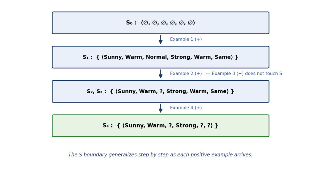
Figure 3: The complete evolution of the S boundary across all four training examples (S₀ → S₁ → S₂, S₃ → S₄).

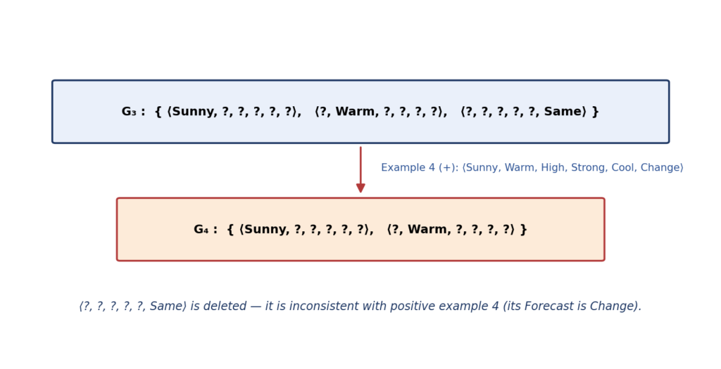
Figure 4: Positive example 4 prunes G₃ — the rule ⟨?, ?, ?, ?, ?, Same⟩ is deleted because it is inconsistent with this positive example.

The Final Version Space

After all four examples, S and G stop moving. This is the final result:

S₄ = { ⟨Sunny, Warm, ?, Strong, ?, ?⟩ }          ← the most specific rule that fits

G₄ = { ⟨Sunny, ?, ?, ?, ?, ?⟩, ⟨?, Warm, ?, ?, ?, ?⟩ }   ← the two most general rules that fit

Think of S as the floor and G as the ceiling. Any rule that sits between them — tighter than the ceiling, looser than the floor — is also a valid answer.

How to Find the Middle Rules

Relax S₄ one constraint at a time. S₄ has three real constraints: Sunny, Warm, Strong:

• Remove “Warm”  → ⟨Sunny, ?, ?, Strong, ?, ?⟩

• Remove “Strong” → ⟨Sunny, Warm, ?, ?, ?, ?⟩

• Remove “Sunny” → ⟨?, Warm, ?, Strong, ?, ?⟩

The complete version space for the EnjoySport concept learning problem therefore contains six hypotheses:

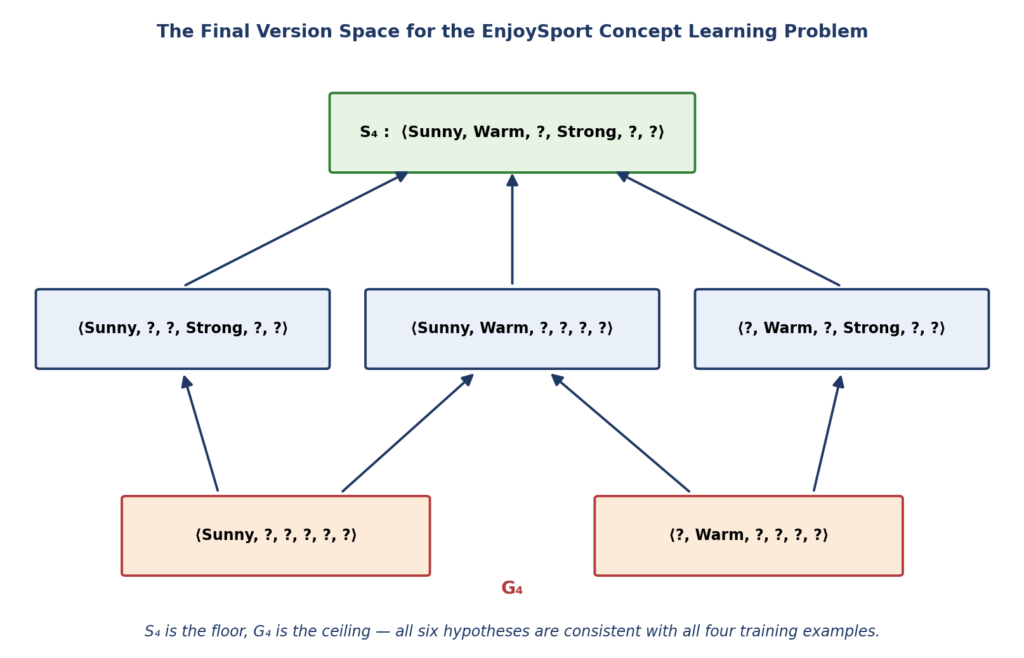
Figure 5: The final version space for the EnjoySport concept learning problem — six hypotheses, with S₄ as the floor and G₄ as the ceiling.

Every hypothesis in this diagram is consistent with all four training examples. The version space tells us exactly how much uncertainty remains — and any future training example that distinguishes between these six hypotheses would narrow it further, until S = G and the concept is found.

Key Takeaways

• CEA maintains the entire version space compactly via just two boundary sets, S and G.

• Positive examples generalize S and prune G; negative examples specialize G and prune S.

• Until the first negative example arrives, CEA’s S boundary behaves identically to FIND-S.

• When S = G, the target concept has been exactly identified; while S ≠ G, the space between them measures the remaining uncertainty.

@SSRoy

REGRESSION-BASIC PREREQUISITE KNOWLEDGE

Statistics and Matrix Algebra Required for Regression

Reference: N. R. Draper and H. Smith, Applied Regression Analysis, 3rd Edition, Chapter 0

@ S. S. Roy   |   Date: 23 July 2026

1. Introduction

Regression analysis requires a fixed set of statistical and matrix tools. Fitting a line is only the first step; every subsequent question — whether a slope is significantly different from zero, how wide its confidence interval is, whether the model as a whole explains anything — is answered using the three distributions, the estimation–testing framework, and the matrix algebra summarised in this tutorial. Each concept is defined below together with its application in regression, before being treated in detail in its own section.

Concept	Definition	Application in regression
Degrees of freedom (df, ν)	The number of independent pieces of information remaining after parameters have been estimated from the data: df = n − (number of estimated parameters).	Determines which t-curve is used for tests and intervals; F requires two df values.
Normal distribution N(μ, σ²)	A symmetric bell-shaped distribution fully determined by its mean μ and standard deviation σ.	The random errors ε in the regression model are assumed normal; this assumption underlies all t and F procedures.
Gamma function Γ(q)	A generalisation of the factorial to non-integer arguments, defined by an integral and satisfying Γ(q) = (q−1)Γ(q−1).	Appears as the normalising constant inside the t and F density formulas; it is evaluated, never integrated, in practice.
t-distribution t(ν)	A family of bell-shaped distributions, one for each df value ν, with heavier tails than the normal; t(∞) = N(0,1).	Confidence intervals and significance tests for individual regression coefficients when σ is estimated by s.
F-distribution F(m, n)	The distribution of a ratio of two independent variance estimates, indexed by two df values; non-negative and right-skewed.	Testing equality of two variances; the overall significance test of a regression model (upper-tailed).
Confidence interval / t-test	Interval: estimate ± t × standard error. Test: t = (estimate − test value) / standard error.	Applied to the slope β₁, the intercept β₀, and predicted responses.
Matrix algebra	Rules for rectangular arrays: transpose, multiplication, inverse, determinant.	Multiple regression is written and solved entirely in matrix form, Y = Xβ + ε, b = (X′X)⁻¹X′Y.

2. Degrees of Freedom

Definition. Degrees of freedom (df, denoted ν) is the number of values in a calculation that are free to vary after certain quantities have been estimated from the same data. Each parameter estimated from the data removes one degree of freedom:

df  =  n  −  (number of parameters estimated from the data)

Example. Consider 5 numbers whose mean is known to be 10, so that their total must equal 50. Any 4 of the numbers can be chosen freely, but the 5th is then forced to whatever value makes the total 50. Five numbers with one estimated quantity (the mean) therefore carry 5 − 1 = 4 degrees of freedom.

Example in regression. A straight-line fit Y = b₀ + b₁X estimates two parameters from the data. With n = 5 observations, the residuals carry n − 2 = 3 degrees of freedom, and the estimate s of σ is said to be based on 3 df.

• Interpretation: df measures the amount of independent information available for estimating the error variance σ². Larger df produces a more reliable s and a t-curve closer to the normal.
• The t-distribution carries one df value (ν). The F-distribution carries two — one for the variance estimate in the numerator, one for the denominator — because each estimate has its own df.

3. The Normal Distribution

Definition. The normal distribution is a symmetric, bell-shaped probability distribution determined completely by two quantities: the mean μ (centre) and the standard deviation σ (spread). Practically the entire distribution (99.73%) lies inside the range μ − 3σ ≤ x ≤ μ + 3σ. The frequency function is:

Application. The normal distribution occurs frequently in the natural world, either for data as they come or for transformed data; the heights of a large randomly selected group of people are approximately normal. In regression, the random errors ε are assumed to be normally distributed — this assumption is what justifies the t and F procedures of later sections.

Notation. x ~ N(μ, σ²) is read “x is normally distributed with mean μ and variance σ².” Most manipulations are carried out with the standard (unit) normal N(0, 1), for which μ = 0 and σ = 1. A general normal variable x is converted to a standard normal variable z by :

z expresses distance from the mean in units of standard deviations. The total area under every normal curve equals 1.

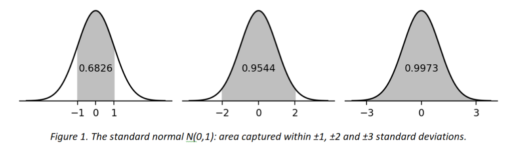
Figure 1. The standard normal N(0,1): area captured within ±1, ±2 and ±3 standard deviations.

Standard areas of the N(0, 1) distribution:

Range of z	Area inside	Area in each tail	Interpretation
−1 to +1	0.6826	0.1587	≈ 68% of the distribution
−2 to +2	0.9544	0.0228	≈ 95%
−3 to +3	0.9973	0.00135 *	“practically all”
−1.645 to +1.645	0.90	0.05	90% limits
−1.96 to +1.96	0.95	0.025	95% limits
−2.57 to +2.57	0.99	0.005	99% limits

* 0.00135 = (1 − 0.9973)/2. All values in this table are obtainable from a standard normal table.

4. The Gamma Function

Definition. The gamma function Γ(q) is a generalisation of the factorial to non-integer arguments. Formally it is defined by the integral:

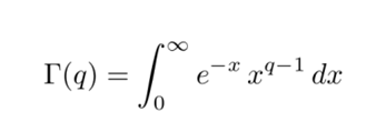
Application. Γ(q) occurs inside the density formulas of the t-distribution (0.1.3) and the F-distribution (0.1.4), where it acts as the normalising constant that makes the total area under each curve equal to 1. In those applications the arguments are integers or half-integers, so the integral is never evaluated directly — the recursion below reduces every case to a simple product.

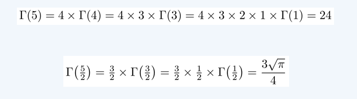
Working rule (generalised factorial property):

Two starting values close the recursion:

Consequently, integer arguments give plain factorials — Γ(n) = (n − 1)! — and half-integer arguments give products ending in √π.

5. The t-Distribution

Definition. The t-distribution is a family of symmetric, bell-shaped distributions, one member for each value of ν, the degrees of freedom. Its density (0.1.3) is:

Application. The t-distribution is used whenever the standard deviation σ is unknown and is estimated by s from the data — the standard situation in regression. Confidence intervals and significance tests for individual regression coefficients (Sections 7–9) are all based on t(ν), where ν is the df of the estimate s.

Shape. A t(ν) curve resembles the standard normal but is heavier in the tails and correspondingly lower in the middle, since the total area must remain 1. The heavier tails reflect the additional uncertainty introduced by estimating σ rather than knowing it.

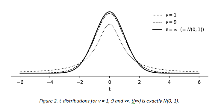
Figure 2. t-distributions for ν = 1, 9 and ∞. t(∞) is exactly N(0, 1).

As ν increases, the distribution becomes more normal; t(∞) is precisely the N(0, 1) distribution. Once ν exceeds about 30, the difference between t(ν) and N(0, 1) is so small that it is conventional — though not mandatory — to use N(0, 1) instead. Regression on small data sets typically has few degrees of freedom, so the t-distribution remains the working tool.

6. The F-Distribution

Definition. The F-distribution is the distribution of a ratio of two statistically independent variance estimates. It depends on two separate degrees of freedom, m (numerator) and n (denominator). Its density (0.1.4) is:

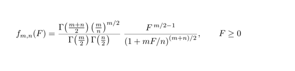
Application. The F-distribution is used to compare two variances, and later to test the overall significance of a regression model. In the standard introduction, the null hypothesis of equal variances is tested against a two-sided alternative:

The test statistic is F = s₁²/s₂², where s₁² and s₂² are statistically independent estimates of σ₁² and σ₂² with ν₁ and ν₂ degrees of freedom respectively. If the two samples are independent and normal, (s₁²/s₂²)/(σ₁²/σ₂²) follows the F(ν₁, ν₂) distribution; hence when σ₁² = σ₂² the plain ratio s₁²/s₂² itself follows F(ν₁, ν₂).

Shape. The distribution is non-negative (it is a ratio of squared quantities), rises from zero — sometimes quite steeply — to a peak, and falls away strongly skewed to the right.

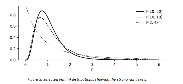
Figure 3. Selected F(m, n) distributions, showing the strong right skew.

One-tailed use in regression: in basic statistics the equal-variance test is two-tailed. In regression applications it is typically a one-tailed, upper-tailed test, because the variance estimate that could be too large — but cannot be too small — is placed in the numerator, and the estimate regarded as a reliable measure of the true σ² is placed in the denominator. The hypotheses are then H₀: σ₁² = σ₂² against H₁: σ₁² > σ₂², and F-tables list upper-tail percentage points at 10%, 5% and 1%.

The three distributions compared

Distribution	Parameters	Shape	Application in regression
Normal N(μ, σ²)	μ and σ	symmetric bell	distributional assumption on the errors ε
t(ν)	one df, ν	bell, heavier tails	intervals and tests for a single coefficient
F(m, n)	two dfs, m and n	non-negative, right-skewed	variance comparison; overall model test

7. Confidence Intervals and t-Tests

Four symbols underlie the entire estimation–testing framework:

Symbol	Name	Meaning
θ	parameter (“thing”)	Any quantity to be estimated — a slope, an intercept, a mean response
θ̂	estimate (“estimate of thing”)	The estimate of θ computed from the data
σ_θ̂	standard deviation of θ̂	The true spread of the estimator; usually unknown, because it contains σ
se(θ̂)	standard error	The estimated standard deviation of θ̂, based on ν degrees of freedom

θ̂ typically follows a normal distribution — either exactly, when the underlying observations are themselves normal, or approximately, by the effect of the Central Limit Theorem. The standard error se(θ̂) is obtained by substituting an estimate of the unknown standard deviation (based on ν degrees of freedom) into the formula for σ_θ̂; this is the reason s replaces σ throughout regression formulas, and the reason a df value accompanies every standard error.

(a) Confidence interval

A 100(1 − α)% confidence interval for θ is given by (0.2.1):

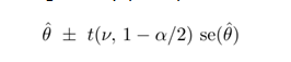
where t(ν, 1 − α/2) is the percentage point of a t-variable with ν degrees of freedom leaving probability α/2 in the upper tail. Equation (0.2.1) in words (0.2.2):

(b) t-Test

To test θ = θ₀, where θ₀ is a specified value presumed valid (θ₀ = 0 in most tests of regression coefficients), the statistic (0.2.3) is evaluated:

or, in words (0.2.4):

The observed t is placed on the t(ν) curve; the tail probability beyond it, δ, is evaluated and doubled for a two-tailed test. The doubled area 2δ is the p-value: the observed value could just as well have come out negative, and the mirror-image point supplies the second δ.

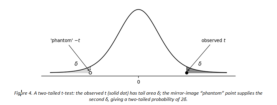
Figure 4. A two-tailed t-test: the observed t (solid dot) has tail area δ; the mirror-image “phantom” point supplies the second δ, giving a two-tailed probability of 2δ.

Decision convention: if 2δ < 0.05, t is termed significant and the hypothesis θ = θ₀ is rejected; if 2δ > 0.05, t is non-significant and the hypothesis is not rejected. The alternative hypothesis is θ ≠ θ₀, a two-sided alternative.

On the significance level α: the value 0.05 is a convention, not an absolute standard. Using α = 0.05 means accepting a 1-in-20 risk of a wrong decision; α = 0.10 (1 in 10) or α = 0.01 (1 in 100) are equally legitimate choices, provided the chosen level is applied consistently throughout the testing. A result at 2δ = 0.049 versus one at 0.051 differs only by an arbitrary boundary; promising experimental leads deserve follow-up even when the arbitrary standard has not quite been attained. The α value is a guidepost, not a boundary.

(c) Applications of formulas (0.2.1)–(0.2.4) — Table 0.1

Every application of the four formulas requires identifying θ, θ̂, θ₀, se(θ̂) and the t percentage point; the formulas themselves never change. The cases arising in the straight-line model Y = β₀ + β₁X + ε are:

Situation	θ	θ̂	se(θ̂)
Slope of the line	β₁	b₁	s / S_XX^½
Intercept of the line	β₀	b₀	s { ΣXᵢ² / (n · S_XX) }^½
Mean response at X = X₀	E(Y) at X₀	Ŷ₀ = b₀ + b₁X₀	s { 1/n + (X₀ − X̄)² / S_XX }^½

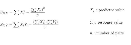
where S_XX = Σ(Xᵢ − X̄)² and s is the estimate of σ obtained from the fit; the symbol s replaces σ of the corresponding standard-deviation formulas. All three standard errors are s multiplied by a quantity built from the X-values.

8. Elements of Matrix Algebra

Definition. Matrix algebra is the arithmetic of rectangular arrays of numbers. Application. Multiple regression with several predictors is formulated and solved entirely in matrix form; the transpose, product, inverse and determinant defined below are precisely the operations used in the estimation formula b = (X′X)⁻¹X′Y and in the construction of confidence regions.

(a) Vocabulary

Term	Meaning	Example
Matrix	A rectangular array with p rows and q columns (a p × q matrix)	A = [[4, 1, 3, 7], [−1, 0, 2, 2], [6, 5, −2, 1]] is 3 × 4
Row vector	A matrix with only one row	a′ = [1, 6, 3, 2, 1], length five
Column vector	A matrix with only one column	b = (−1, 0, 1)′, length three
Scalar	A 1 × 1 “vector” — an ordinary number	7

Convention (not universal): capital letters denote matrices, lower-case letters denote vectors, often in boldface; brackets may be square-ended or curved. The plural of matrix is matrices.

(b) Basic operations

Operation	Rule	Condition
Equality	Identical entry in every position	Dimensions must be identical
Sum / Difference	Element-by-element addition or subtraction	Dimensions must be identical, otherwise undefined
Transpose (M′)	Rows of M become the columns of M′, in the same order	Always defined
Symmetry	M is symmetric if M′ = M	M must be square
Multiplication (AB)	cᵢⱼ = Σ aᵢₗ bₗⱼ — the inner product of row i of A with column j of B	A is p × q, B must be q × s (conformable); result is p × s

Multiplication example — a 2 × 3 matrix times a 3 × 3 matrix gives a 2 × 3 result:

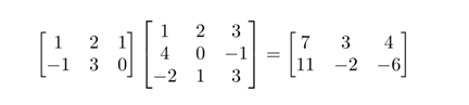
Verification of the top-left entry: 1(1) + 2(4) + 1(−2) = 7. Every other entry is the corresponding row-by-column inner product.

Two properties of matrix multiplication: (1) AB and BA, even when both are conformable, do not in general give the same result — the order of matrices is crucial, unlike the order of numbers in a scalar product. In AB, B is premultiplied by A, equivalently A is postmultiplied by B. (2) When several matrices and vectors are multiplied together, the bracketing that leads to the least work should be chosen: for W(p×p) Z′(p×n) y(n×1), computing W(Z′y) requires far fewer cross-products than (WZ′)y.

(c) Special matrices and vectors

Symbol	Name	Content	Role
Iₙ	Identity (unit) matrix	n × n, 1s on the diagonal, 0s elsewhere	The matrix counterpart of the number 1; the subscript n is omitted when the size is clear
0	Zero vector or matrix	Every entry zero	The counterpart of the number 0; size clear from context
1	Vector of ones	(1, 1, …, 1)′	1′1 equals the squared length of 1; 11′ is a square matrix of all 1s

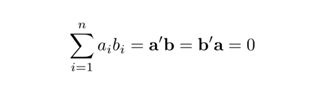
Orthogonality. A vector a = (a₁, …, aₙ)′ is orthogonal to a vector b = (b₁, …, bₙ)′ if the sum of the products of their elements is zero:

(d) Inverse matrix

Definition. The inverse M⁻¹ of a square matrix M is the unique matrix satisfying:

Existence depends on linear dependence: the columns m₁, m₂, …, mₙ of an n × n matrix are linearly dependent if there exist constants c₁, c₂, …, cₙ, not all zero, such that

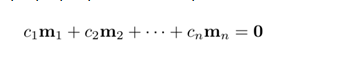
and similarly for rows. Then:

• A square matrix with linearly dependent rows or columns is singular and possesses no inverse. A square matrix that is not singular is nonsingular and can be inverted.
• If M is symmetric, so is M⁻¹. (In regression, the matrix to be inverted, X′X, is always symmetric.)

Obtaining an inverse

The inversion procedure is defined through an example. To invert M = [3 4 5 ; 1 2 6 ; 7 1 9], M⁻¹ is written as a matrix of nine unknowns (a, b, c, …, h, k) subject to M⁻¹M = I:

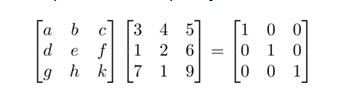
Multiplying out and matching every entry against I produces three sets of three linear simultaneous equations — one set per column of unknowns:

Solving the nine equations yields the inverse (with the common factor 1/103 removed, as described in Section (f)):

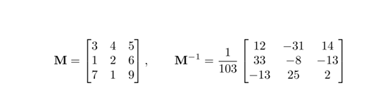
For an n × n matrix there are, in general, n sets of n simultaneous linear equations. Accelerated methods adapted for computers obtain inverses with great speed even for large matrices; hand inversion is obsolete except in simple cases such as the 2 × 2 formula:

Determinant route to the inverse (verifiable against the 2 × 2 formula above): replace each element mᵢⱼ of M by (1) the determinant of the submatrix obtained by crossing out the row and column containing mᵢⱼ, (2) with the sign attached from the + − + − count, (3) divided by det M. When every element has been replaced, the resulting matrix is transposed; that transpose is M⁻¹.

(e) Determinants

Definition. The determinant is a single number associated with a square matrix. Determinants occur naturally in the solution of linear simultaneous equations and in the inversion of matrices. For a 2 × 2 matrix:

For a 3 × 3 matrix [a b c ; d e f ; g h k], expanding by the first row — each first-row element multiplied by the determinant of the submatrix left after crossing out its row and column, with alternating signs + − + — gives:

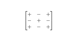
The determinant can be written as an expansion of any row or column by the same technique. The signs attached are counted + − + − from the top left-hand corner element, alternating along a row or column (not diagonally):

Geometrically, the determinant measures the volume of the parallelepiped defined by the vectors in the rows (or columns) of the matrix; this is the reason det(X′X) later determines the size of a joint confidence region for regression parameters.

(f) Common factors

If every element of a matrix has a common factor, it can be taken outside the matrix; conversely, multiplying a matrix by a constant c multiplies every element by c:

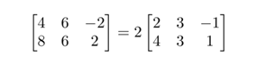
Determinant of a scaled matrix: for a square p × p matrix with common factor c, the determinant carries the factor cᵖ, not c:

9. Solved Example 1 — Confidence Interval and t-Test on a Fitted Line

X	0	1	2	3	4
Y	3	6	8	11	12

Solution

Step 1 — means. X̄ = (0+1+2+3+4)/5 = 2,   Ȳ = (3+6+8+11+12)/5 = 40/5 = 8.

Step 2 — sums of squares and products (deviations from the means):

Xᵢ − X̄	−2	−1	0	1	2	Sum
Yᵢ − Ȳ	−5	−2	0	3	4	—
(Xᵢ − X̄)²	4	1	0	1	4	S_XX = 10
(Xᵢ − X̄)(Yᵢ − Ȳ)	10	2	0	3	8	S_XY = 23

Step 3 — fitted line. b₁ = S_XY / S_XX = 23/10 = 2.3, and b₀ = Ȳ − b₁X̄ = 8 − 2.3(2) = 3.4:

Step 4 — estimate s of σ. Fitted values and residuals:

X	0	1	2	3	4
Ŷ = 3.4 + 2.3X	3.4	5.7	8.0	10.3	12.6
Residual (Y − Ŷ)	−0.4	0.3	0.0	0.7	−0.6
Residual²	0.16	0.09	0.00	0.49	0.36

The sum of squared residuals is 1.10 on n − 2 = 3 degrees of freedom (two df are removed by the estimation of b₀ and b₁; compare Section 2). Therefore:

Step 5 — standard error of the slope. From Table 0.1:

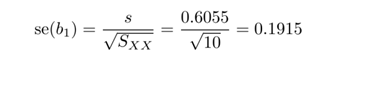
Step 6 — 95% confidence interval, formula (0.2.1). With α = 0.05 and ν = 3, the t-table gives t(3, 0.975) = 3.182:

Interpretation: with 95% confidence, the true slope lies between 1.69 and 2.91. The interval is wide because at only 3 degrees of freedom the t-multiplier 3.182 is far larger than the large-sample value 1.96.

Step 7 — t-test of H₀: β₁ = 0, formula (0.2.3). Here θ̂ = 2.3 and θ₀ = 0:

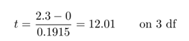
Since |12.01| exceeds the critical value 3.182, the result is significant at the 5% level (exact two-tailed probability 2δ ≈ 0.0012). H₀ is rejected: the slope is non-zero, and X contributes genuinely to the explanation of Y.

Relationship between interval and test: the confidence interval (1.69, 2.91) excludes 0, and the t-test rejects β₁ = 0. The two procedures always agree in this way — a two-sided t-test at level α rejects θ = θ₀ exactly when the 100(1−α)% confidence interval excludes θ₀.

10. Solved Example 2 — The Same Fit in Matrix Form

Problem. For the three points X = 1, 2, 3 with Y = 2, 4, 5: set up the matrices X and Y; compute X′X, its determinant and inverse; obtain the coefficient vector b = (X′X)⁻¹X′Y; and verify the result against the ordinary least-squares formulas.

Solution

Step 1 — matrices. The column of 1s carries the intercept:

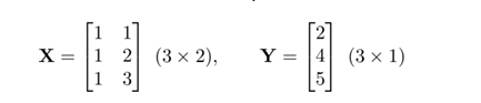
Step 2 — transpose and product. X′ is 2 × 3, so X′X is conformable and yields a 2 × 2 result:

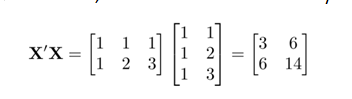
Entry by entry: top-left = 1+1+1 = 3 (which is n); top-right = 1+2+3 = 6 (ΣX); bottom-right = 1+4+9 = 14 (ΣX²). X′X is symmetric, in agreement with Section 8(d).

Step 3 — determinant. det(X′X) = (3)(14) − (6)(6) = 42 − 36 = 6. The determinant is non-zero, so the matrix is nonsingular and invertible.

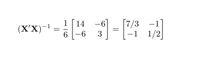
Step 4 — inverse, by the 2 × 2 formula. Diagonal entries swapped, off-diagonal entries negated, all divided by the determinant:

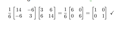
Verification — the product with the original matrix must return I:

Step 5 — X′Y.

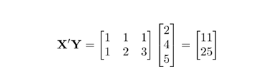
Step 6 — coefficients.

Hence b₀ = 0.667 and b₁ = 1.5, giving Ŷ = 0.667 + 1.5X.

Step 7 — cross-check with the ordinary formulas. X̄ = 2, Ȳ = 11/3. S_XX = 1 + 0 + 1 = 2 and S_XY = (−1)(−5/3) + 0 + (1)(4/3) = 3. Then b₁ = 3/2 = 1.5 and b₀ = 11/3 − 1.5(2) = 0.667. The matrix route and the scalar route agree exactly.

Purpose of the matrix formulation: the formula b = (X′X)⁻¹X′Y belongs to a later chapter; it is included here to show where the transpose, conformability, symmetry, determinant and inverse of Section 8 are applied. With one predictor the matrix route duplicates the scalar formulas; with many predictors it is the only practical method, and every step remains identical — only the matrix dimensions grow.

11. One-Page Recap

Idea	Summary
Degrees of freedom	df = n − (parameters estimated); measures independent information; t carries one df, F carries two
Normal	Symmetric; z = (x − μ)/σ; ±1σ → 68%, ±2σ → 95%, ±3σ → 99.7%; ±1.96 → exactly 95%; assumption on the errors ε
Gamma	Γ(q) = (q−1)Γ(q−1), with Γ(1) = 1 and Γ(½) = √π; the normalising constant inside t and F densities
t-distribution	One df ν; heavier-tailed than the normal; t(∞) = N(0,1); used whenever σ is estimated by s
F-distribution	Two dfs; non-negative, right-skewed; ratio of two variance estimates; upper-tailed in regression
Confidence interval	estimate ± t(ν, 1−α/2) × standard error
t-test	t = (estimate − test value) / standard error; doubled tail area 2δ is the p-value; compare with α
Significance level	α = 0.05 is a convention — a guidepost, not a boundary
Matrix multiplication	A(p×q) B(q×s) defined only when inner dimensions match; result p×s; AB ≠ BA in general
Transpose / symmetry	M′ interchanges rows and columns; M symmetric if M′ = M; X′X is always symmetric
Inverse	M⁻¹M = I; exists only for square nonsingular matrices (det ≠ 0); found from n sets of n simultaneous equations, or by the determinant route
Determinant	2×2: ad − bc; expansion along any row or column with + − + signs; common factor c emerges as cᵖ

Next step: with these tools in place, the straight-line model Y = β₀ + β₁X + ε can be developed — least-squares fitting, t-tests on the coefficients, an F-test on the whole model, and the generalisation to many predictors in the matrix form Y = Xβ + ε.

Exercise Problem.

The breaking strength of steel rods is normally distributed. A sample of n = 8 rods gives a sample mean X̄ = 52 units and a sample standard deviation s = 4 units. For the process as a whole, the true values are known historically to be μ = 50 and σ = 4.

(a) State the degrees of freedom associated with s.
(b) Using the historical values, find the z-score of a rod measuring 58 units, and the proportion of rods measuring between 42 and 58 units.
(c) Evaluate Γ(4) and Γ(7/2).
(d) Using the sample results, construct a 95% confidence interval for the true mean μ.

Solution

(a) Degrees of freedom. One parameter (the mean) is estimated from the data, so one degree of freedom is lost:

df = n − 1 = 8 − 1 = 7

(b) Normal distribution. With μ = 50 and σ = 4, apply z = (x − μ)/σ:

z at x = 58 → (58 − 50)/4 = +2
z at x = 42 → (42 − 50)/4 = −2

The range 42 to 58 is exactly ±2σ about the mean. From the standard normal table, the area between z = −2 and z = +2 is 0.9544, so approximately 95.44% of rods lie between 42 and 58 units.

(c) Gamma function. Apply Γ(q) = (q − 1)Γ(q − 1) with Γ(1) = 1 and Γ(½) = √π.

Γ(4) = 3 × Γ(3) = 3 × 2 × Γ(2) = 3 × 2 × 1 × Γ(1) = 6 (= 3!)
Γ(7/2) = (5/2) × (3/2) × (1/2) × Γ(1/2) = 15√π / 8 ≈ 3.3234

(d) t-distribution — 95% confidence interval. Since σ is estimated by s, the t-distribution applies with ν = 7 df. The standard error is:

se(X̄) = s/√n = 4/√8 = 1.4142

From the t-table, t(7, 0.975) = 2.365. Applying the interval formula:

52 ± 2.365 × 1.4142 = 52 ± 3.34 = (48.66, 55.34)

Note the effect of small df: the multiplier 2.365 is appreciably larger than the large-sample normal value of 1.96, which widens the interval.

---

Practice Exercises (keys only)

Exercise 1. A straight line Y = β₀ + β₁X is fitted to n = 12 observations. (a) State the df of the estimate s. (b) Evaluate Γ(6). (c) State the t multiplier for a 95% confidence interval on β₁. (d) Compare it with the corresponding normal value.

Key: (a) 12 − 2 = 10 df (two parameters estimated). (b) Γ(6) = 5! = 120. (c) t(10, 0.975) = 2.228. (d) Larger than 1.96; the gap narrows as df increases.

Exercise 2. Examination marks follow N(60, 8²). (a) Find the z-score of a student scoring 76. (b) Find the percentage of students scoring between 44 and 76. (c) Find the mark exceeded by only 2.5% of students. (d) Evaluate Γ(9/2).

Key: (a) z = (76 − 60)/8 = +2. (b) 44 gives z = −2, so the range is ±2σ → 95.44%. (c) Upper 2.5% corresponds to z = 1.96, so mark = 60 + 1.96(8) = 75.68. (d) Γ(9/2) = (7/2)(5/2)(3/2)(1/2)√π = 105√π/16 ≈ 11.6317.

Exercise 3. A sample of n = 25 observations gives X̄ = 100 and s = 10. (a) State the df. (b) Compute se(X̄). (c) Construct a 95% confidence interval for μ, given t(24, 0.975) = 2.064. (d) State which distribution and which multiplier would apply if σ = 10 were known instead of estimated.

Key: (a) 25 − 1 = 24 df. (b) se(X̄) = 10/√25 = 2. (c) 100 ± 2.064(2) = 100 ± 4.13 = (95.87, 104.13). (d) The standard normal N(0, 1), multiplier 1.96 — giving the narrower interval (96.08, 103.92).

LEAST SQUARES ESTIMATION

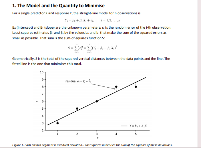
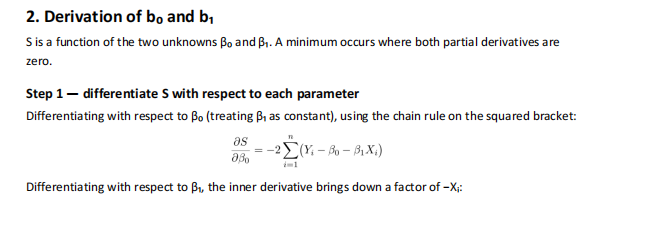
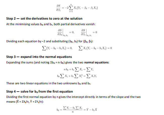
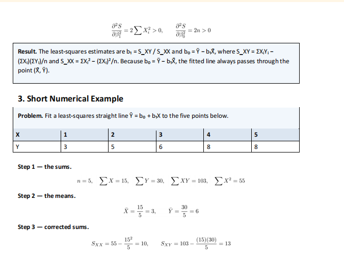
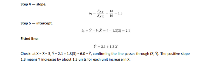
Derivation of the Estimates b₀ and b₁ for a Straight Line

Reference: N. R. Draper and H. Smith, Applied Regression Analysis, 3rd Edition, Chapter 1

MULTIPLE LINEAR REGRESSION

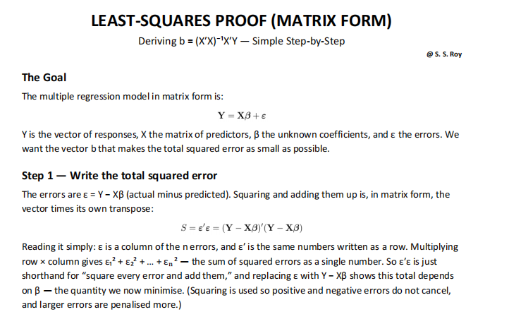
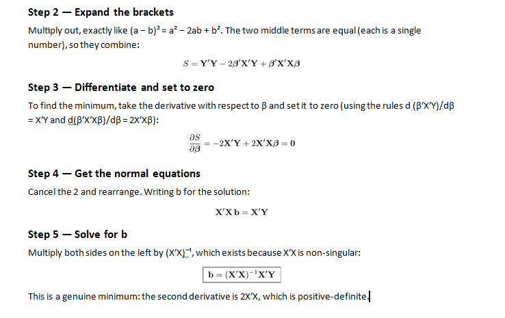
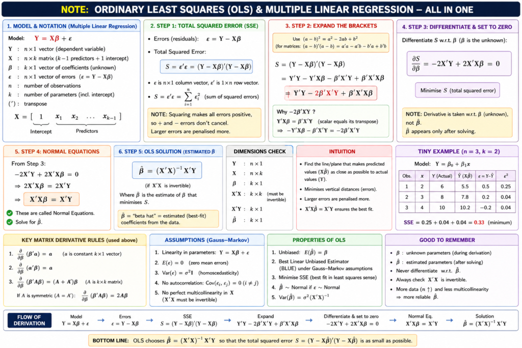
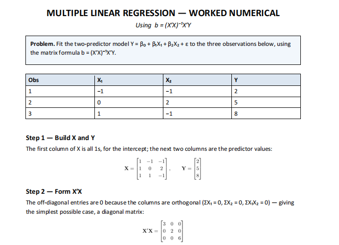
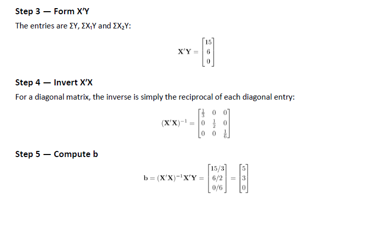
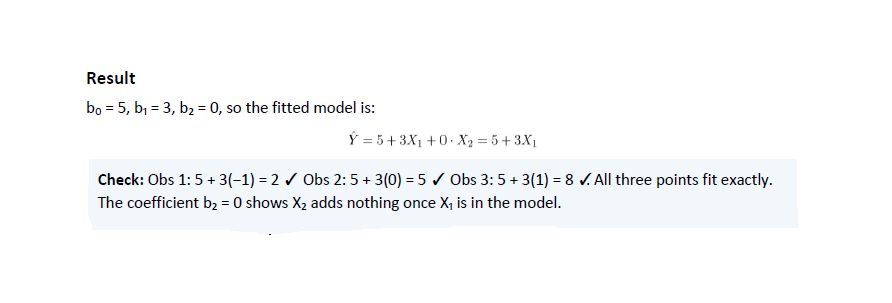
Direct Visual Comparison

• Single Linear Regression Graph: A 2D scatter plot where a straight line passes through a cloud of data points.
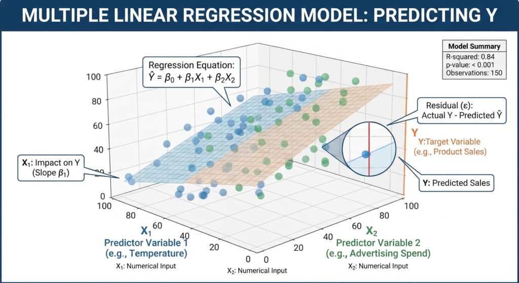
• Multiple Linear Regression Graph: A 3D scatter plot where a flat plane cuts through a cloud of data points (for two predictors), or a series of separate 2D lines (for three or more predictors)

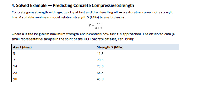
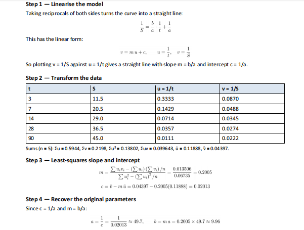
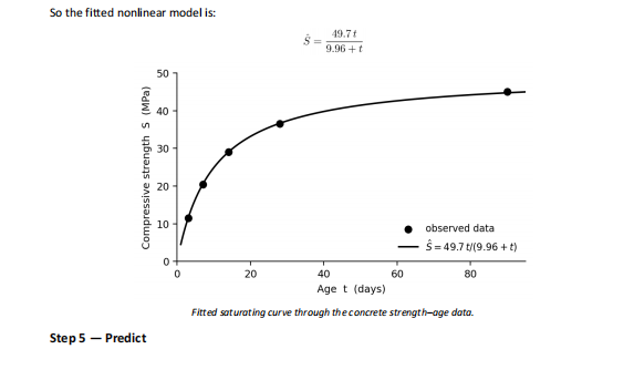
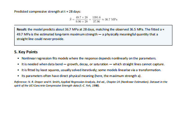
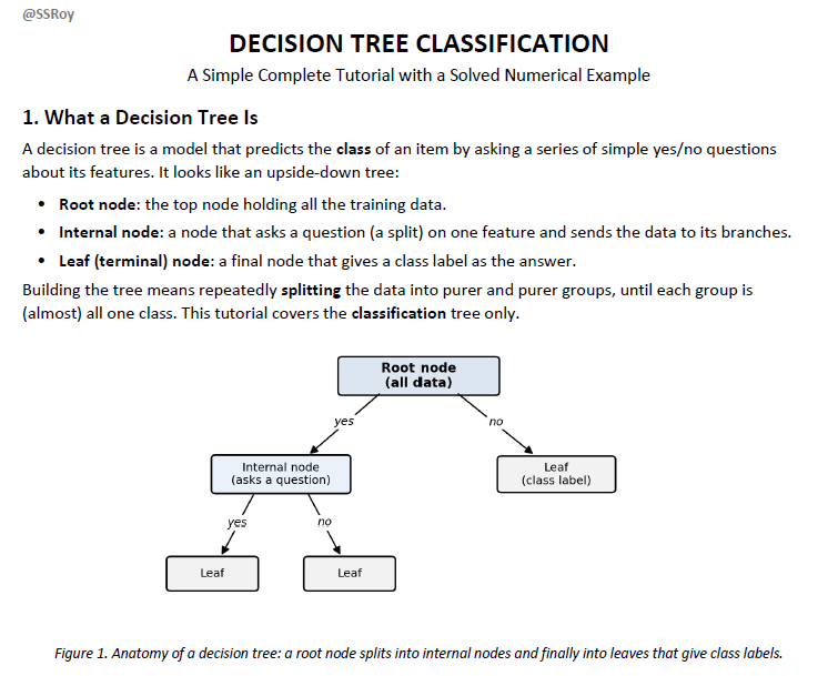
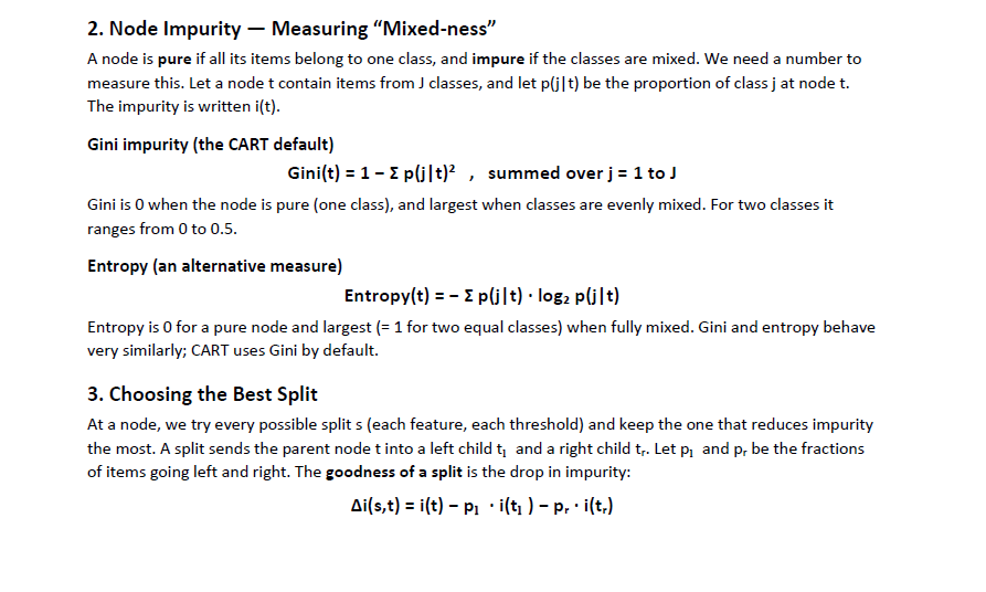
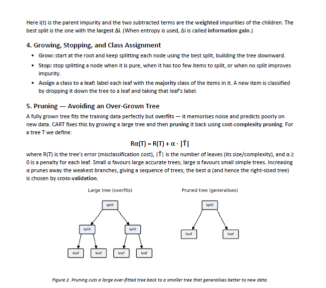
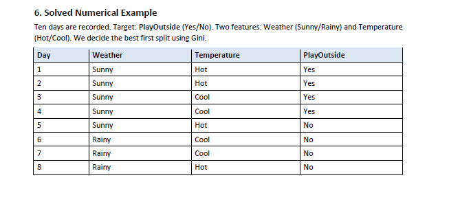
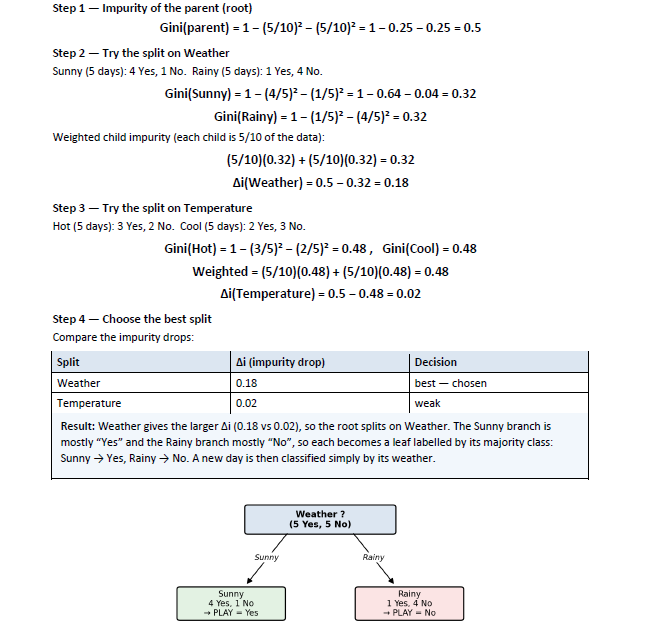
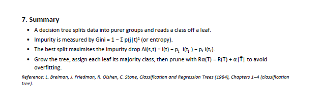
Solved Numerical Example — Decision Tree (Gini)

Problem. A bank wants to predict Loan Approved (Yes/No) from two features: Credit Score (High/Low) and Income (High/Low). Using the 8 records below, decide the best feature for the first split using Gini impurity.

Training data

Applicant	Credit Score	Income	Loan Approved
1	High	High	Yes
2	High	Low	Yes
3	High	High	Yes
4	High	Low	Yes
5	Low	High	No
6	Low	Low	No
7	Low	High	Yes
8	Low	Low	No

Class counts: 5 Yes, 3 No out of 8.

Formula used

Gini(t) = 1 − Σ p(j|t)² (impurity of a node)
Δi = Gini(parent) − [ p_L·Gini(left) + p_R·Gini(right) ] (impurity drop)

Pick the split with the largest Δi.

Step 1 — Impurity of the parent (root)

Gini(parent) = 1 − (5/8)² − (3/8)² = 1 − 0.3906 − 0.1406 = 0.4688

Step 2 — Try the split on Credit Score

Credit = High (4 records): 4 Yes, 0 No → pure node
Credit = Low (4 records): 1 Yes, 3 No

Gini(High) = 1 − (4/4)² − (0/4)² = 1 − 1 − 0 = 0
Gini(Low) = 1 − (1/4)² − (3/4)² = 1 − 0.0625 − 0.5625 = 0.375

Weighted child impurity (each child is 4/8 = ½ of the data):

(4/8)(0) + (4/8)(0.375) = 0.1875
Δi(Credit) = 0.4688 − 0.1875 = 0.2813

Step 3 — Try the split on Income

Income = High (4 records): 3 Yes, 1 No
Income = Low (4 records): 2 Yes, 2 No

Gini(High) = 1 − (3/4)² − (1/4)² = 0.375
Gini(Low) = 1 − (2/4)² − (2/4)² = 0.5

Weighted child impurity:

(4/8)(0.375) + (4/8)(0.5) = 0.4375
Δi(Income) = 0.4688 − 0.4375 = 0.0313

Step 4 — Choose the best split

Split	Δi (impurity drop)	Decision
Credit Score	0.2813	best — chosen
Income	0.0313	weak

Result: Credit Score gives the far larger impurity drop (0.28 vs 0.03), so the root splits on Credit Score. The Credit = High branch is pure (all Yes) and becomes a leaf → Approved = Yes. The Credit = Low branch (1 Yes, 3 No) becomes a leaf by majority → Approved = No. A new applicant is classified simply by their credit score.

Resulting tree:

              Credit Score?
             /            \
          High             Low
       (4Y, 0N)         (1Y, 3N)
     Approved = Yes    Approved = No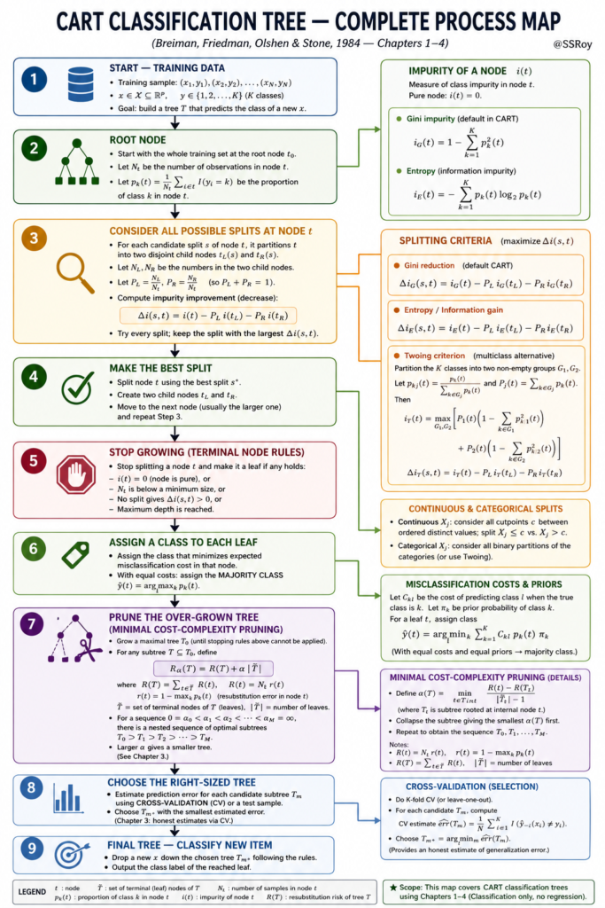

Support Vector Machine