Course notes — @ S. S. Roy
0. The whole idea in one paragraph
In supervised learning somebody hands you the right answer and you copy it. In reinforcement learning nobody knows the right answer. You act, the world scores you, and you get better. That’s it. Everything below — Bellman equations, TD learning, Q-learning, actor–critic — is machinery for doing that scoring efficiently.
PART I — Where the idea comes from
1. You already learned this way
The familiar machine learning models learn from data: here are labelled examples, imitate them. That is learning by instruction.
Now ask yourself: how did you learn to cycle?
- By trial and error.
- Falling down hurts.
- Nobody told you the correct handlebar angle at each instant.
- You got evaluation, not instruction.
That is reinforcement learning. Same for learning to walk, and learning to talk.
So RL is:
- a trial-and-error learning paradigm
- driven by reward and punishment
- a way to learn about anything through interaction
- inspired by behavioural psychology
2. Pavlov’s dog — where the reward signal comes from
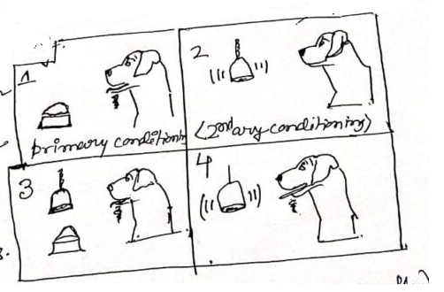
While studying digestion in dogs, Ivan Pavlov stumbled onto classical conditioning: a neutral stimulus becomes associated with a meaningful one.
| Stage | What is presented | What the dog does |
|---|---|---|
| Before | Food | Salivates — natural reflex |
| Bell | Nothing | |
| During | Bell rung just before food, many times | Salivates (to the food) |
| After | Bell alone | Salivates |
The dog learned to associate the bell (neutral) with food (unconditioned stimulus), and eventually responded to the bell by itself. The bell had become a conditioned stimulus.
That association-by-experience is the biological ancestor of the reward signal.
3. Why bother with RL at all?
- Large language models. ChatGPT is the recent, famous case.
- Complex dynamics. Helicopter control — too intricate to program by hand.
- Complex workspaces. Too large or unstructured to enumerate.
- Stochastic sensing and actuation. Sensors are noisy; actuators don’t do exactly what they’re told.
The common thread: nobody can write down the right action for every situation in advance. The system has to find it.
PART II — The vocabulary
4. Definition
Reinforcement Learning is a branch of machine learning concerned with how an agent ought to take actions in an environment so as to maximise cumulative reward.
More formally:
A computational approach to goal-directed learning and decision making in which an agent learns to achieve goals through interaction with an environment, by receiving evaluative feedback (rewards) about its actions rather than explicit instructions.
Three ways it differs from supervised learning:
| Supervised learning | Reinforcement learning | |
|---|---|---|
| Feedback | The correct label | A number saying how good that was |
| Timing | Immediate | Often delayed |
| Data | Fixed dataset | Generated by your own actions |
That third row is the one people underestimate. In RL your data depends on your policy, and your policy depends on your data. That loop is the whole difficulty.
5. The interaction loop
[FIGURE — agent–environment loop, from your handwritten notes]
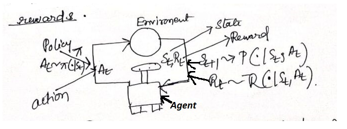
At each time step t:
- The agent observes a state Sₜ
- It takes an action Aₜ
- It receives a reward Rₜ₊₁
- The environment moves to a new state Sₜ₊₁
with
Sₜ₊₁ ~ P(· | Sₜ, Aₜ) and Rₜ₊₁ ~ R(· | Sₜ, Aₜ)
| Component | Role |
|---|---|
| Agent | The learner / decision-maker |
| Environment | Everything the agent interacts with |
| Reward signal | Numerical feedback on the value of an outcome |
6. Five symbols that carry the whole subject
| Symbol | Name | Plain English |
|---|---|---|
| π(a|s) | policy | The agent’s behaviour — what it does in each state |
| Gₜ | return | Total discounted reward from now to the end |
| v(s) | state value | “How good is it to be here?” |
| q(s,a) | action value | “How good is it to do this, here?” |
| γ | discount factor | How much I care about the future |
The return:
Gₜ = Rₜ₊₁ + γRₜ₊₂ + γ²Rₜ₊₃ + … = Σ_{k=0}^{∞} γᵏ R_{t+k+1}
The value functions:
v_π(s) = 𝔼_π[ Gₜ | Sₜ = s ] and q_π(s,a) = 𝔼_π[ Gₜ | Sₜ = s, Aₜ = a ]
Why γ? Two reasons. Mathematically, with 0 ≤ γ < 1 an infinite sum of bounded rewards stays finite. Intuitively, a reward now is worth more than the same reward later. γ = 0 is a pure short-termist; γ → 1 is infinitely patient.
7. Key features of RL, restated
- Sequential decision-making — each action shapes the situations you face later
- No direct supervision — you learn by trial and error
- Goal-directed behaviour — cumulative reward is the objective, not per-step accuracy
- Environmental feedback — often delayed, often sparse
PART III — One problem, solved six ways
Everything from here on uses the same tiny problem. Learn it once and every algorithm becomes a variation on a theme you already know.
8. The running example: the two-room robot
A robot lives in two rooms.
From A it moves to B and collects reward +2.
From B it moves back to A and collects reward +1.
Discount γ = 0.5.
There is one action per state for now, so there is only one policy. The only question is: what are these two states worth?
Solving it exactly
Write down what each state is worth: the reward you get right now, plus half of whatever you land in.
v(A) = 2 + 0.5·v(B)
v(B) = 1 + 0.5·v(A)
Substitute the second into the first:
v(A) = 2 + 0.5(1 + 0.5·v(A))
v(A) = 2 + 0.5 + 0.25·v(A)
0.75·v(A) = 2.5
v(A) = 10/3 = 3.3333… v(B) = 8/3 = 2.6667…
Remember those two numbers. Every method below has to find them.
Why this pair is worth memorising: the two lines above are the Bellman equations in miniature. In general:
v_π(s) = Σ_a π(a|s) Σ_{s′,r} p(s′,r|s,a) [ r + γ·v_π(s′) ]
Same statement — reward now, plus discounted value of where you land — just written for many actions and stochastic outcomes.
And when you get to choose the best action rather than follow a fixed policy, the sum over actions becomes a max — the Bellman optimality equations:
v*(s) = max_a Σ_{s′,r} p(s′,r|s,a) [ r + γ·v*(s′) ]
q*(s,a) = Σ_{s′,r} p(s′,r|s,a) [ r + γ·max_{a′} q*(s′,a′) ]
For finite MDPs, these have a unique solution.
The setting has a name
This problem is a finite Markov Decision Process (MDP): the next state and reward depend only on the current state and action, not on anything earlier. That is the Markov property, and it’s what makes all of this tractable.
| Symbol | Meaning |
|---|---|
| 𝒮 | set of states |
| 𝒜(s) | actions available in s |
| p(s′, r | s, a) | dynamics — the transition/reward model |
| π(a | s) | policy |
| γ ∈ [0,1) | discount factor |
Method 1 — Dynamic Programming: I know the rules
Use when: you know p(s′, r | s, a) exactly.
Idea: guess the values, then keep applying the Bellman equation until the guess stops changing.
Policy evaluation:
v_{k+1}(s) = Σ_a π(a|s) Σ_{s′,r} p(s′,r|s,a) [ r + γ·v_k(s′) ]
On the two-room robot
Start from nothing: v₀(A) = v₀(B) = 0. Then just apply the two lines repeatedly.
| Sweep | v(A) | v(B) |
|---|---|---|
| 0 | 0.0000 | 0.0000 |
| 1 | 2 + 0.5(0) = 2.0000 | 1 + 0.5(0) = 1.0000 |
| 2 | 2 + 0.5(1) = 2.5000 | 1 + 0.5(2) = 2.0000 |
| 3 | 2 + 0.5(2) = 3.0000 | 1 + 0.5(2.5) = 2.2500 |
| 4 | 3.1250 | 2.5000 |
| 5 | 3.2500 | 2.5625 |
| 6 | 3.2812 | 2.6250 |
| … | … | … |
| 12 | 3.3325 | 2.6660 |
Crawling toward 3.3333 and 2.6667. ✓
Once you can evaluate, you can improve. Act greedily with respect to the values you just computed:
π′(s) = arg max_a Σ_{s′,r} p(s′,r|s,a) [ r + γ·v_π(s′) ]
Alternate evaluation and improvement → policy iteration. Collapse them into one step → value iteration:
v_{k+1}(s) = max_a Σ_{s′,r} p(s′,r|s,a) [ r + γ·v_k(s′) ]
The catch: DP needs the model. Real robots do not come with p(s′, r | s, a) printed on the box.
Method 2 — Monte Carlo: play it out and average
Use when: you have no model, but episodes end.
Idea: the value of a state is the average return you actually got after visiting it. No theory, just bookkeeping.
V(s) ← average of Gₜ over visits to s
On the two-room robot — with one honest caveat
Monte Carlo cannot run on the robot as specified, because A ↔ B cycles forever and MC needs an episode to finish before it can compute a return. This is not a technicality — it’s the single most important limitation of the method.
So we use the episodic cousin: the robot’s shift ends after room B.
A —(+2)→ B —(+2 or 0, equal chance)→ shift over
Exactly: v(B) = average final reward = 1.0, and v(A) = 2 + 0.5(1) = 2.5.
| Episode | Final reward | G(A) | G(B) |
|---|---|---|---|
| 1 | 0 | 2.0 | 0.0 |
| 2 | 2 | 3.0 | 2.0 |
| 3 | 0 | 2.0 | 0.0 |
| … | |||
| After 20,000 | V(A) = 2.5056 | V(B) = 1.0112 |
Converging on 2.5 and 1.0. ✓
Read the numbers carefully. MC is unbiased — it’s averaging real returns, so it’s aimed at the right target — but it is noisy, and it needs 20,000 episodes to get two decimal places on a problem this trivial. And it learns nothing until an episode finishes.
Method 3 — Temporal-Difference learning: don’t wait, guess
Use when: no model, and you want to learn online, mid-episode, possibly forever.
Idea: MC waits for the true return. TD refuses to wait and substitutes its own current estimate of the next state. This is called bootstrapping.
The gap between what you expected and what the next step suggests is the TD error:
δₜ = R_{t+1} + γ·V(S_{t+1}) − V(Sₜ)
and you nudge your estimate toward it:
V(Sₜ) ← V(Sₜ) + α·δₜ
α is the step size — how much you trust each new piece of evidence.
On the two-room robot
α = 0.1, starting from V(A) = V(B) = 0. Now the robot just walks, and we update as it goes.
| Step | From | R | δ = R + γV(next) − V(here) | Update |
|---|---|---|---|---|
| 0 | A | 2 | 2 + 0.5(0) − 0 = +2.0000 | V(A) → 0 + 0.1(2.0) = 0.2000 |
| 1 | B | 1 | 1 + 0.5(0.2) − 0 = +1.1000 | V(B) → 0.1100 |
| 2 | A | 2 | 2 + 0.5(0.11) − 0.2 = +1.8550 | V(A) → 0.3855 |
| 3 | B | 1 | 1 + 0.5(0.3855) − 0.11 = +1.0827 | V(B) → 0.2183 |
| … | ||||
| 4000 | V(A) = 3.3333, V(B) = 2.6667 |
Exact. ✓
And note what just happened: no model, no episode boundary, updating every single step. That combination is why TD is the workhorse of the field.
MC vs TD, side by side:
| Monte Carlo | TD(0) | |
|---|---|---|
| Waits for | End of episode | One step |
| Works on continuing tasks | ✗ | ✓ |
| Bias | None | Some (bootstraps off its own guess) |
| Variance | High | Low |
| Needs a model | ✗ | ✗ |
Method 4 — TD(λ): spread the credit backwards
Use when: rewards arrive long after the actions that earned them.
Idea: TD(0) only updates the state you just left. But the state before that also deserves some credit. Eligibility traces keep a fading memory of everywhere you’ve recently been, so one surprise updates them all at once.
The trace — bumped on visit, decaying otherwise:
eₜ(s) = γλ·e_{t−1}(s) + 𝟙{Sₜ = s}
The update — every state moves, in proportion to how recently it was seen:
V(s) ← V(s) + α·δₜ·eₜ(s)
λ is the dial. λ = 0 gives you TD(0) back. λ = 1 behaves like Monte Carlo. In between you get n-step methods blended together, which is what the forward view says:
Gₜ^(λ) = (1 − λ) Σ_{n=1}^{∞} λ^{n−1}·Gₜ^(n)
On the two-room robot
λ = 0.8, α = 0.05, same walk: after 4000 steps, V(A) = 3.3333, V(B) = 2.6667. ✓
Same destination as TD(0) — but on problems with long delays between action and reward (mazes, games), traces get there far faster, because a single good outcome propagates back along the whole path immediately instead of one step per episode.
Method 5 — SARSA and Q-Learning: now actually choose
Everything so far answered “what is this worth?” — prediction. Now we do control: choosing the best action.
First, give the robot a choice
Add a second action in room A: IDLE — stay put, earn nothing.
In A:
WORK→ B, reward +2 |IDLE→ A, reward 0
In B:BACK→ A, reward +1
Solve exactly, using v*(A) = 10/3 and v*(B) = 8/3 from before:
| Action value | Calculation | Exact | Decimal |
|---|---|---|---|
| q*(A, WORK) | 2 + 0.5(8/3) | 10/3 | 3.3333 |
| q*(A, IDLE) | 0 + 0.5(10/3) | 5/3 | 1.6667 |
| q*(B, BACK) | 1 + 0.5(10/3) | 8/3 | 2.6667 |
WORK (3.3333) beats IDLE (1.6667), so the optimal policy is to work. Now let’s see whether the algorithms figure that out without being told the rules.
The two update rules
They differ in one term, and that one term is the whole on-policy / off-policy distinction.
SARSA — on-policy. Uses the action you actually took next:
Q(S,A) ← Q(S,A) + α[ R + γ·Q(S′,A′) − Q(S,A) ]
Q-Learning — off-policy. Uses the best available next action, whatever you actually did:
Q(S,A) ← Q(S,A) + α[ R + γ·max_{a′} Q(S′,a′) − Q(S,A) ]
Results on the two-room robot
Both with ε-greedy exploration (ε = 0.1), α = 0.1, learning from experience alone:
| Q(A,WORK) | Q(A,IDLE) | Q(B,BACK) | Greedy choice in A | |
|---|---|---|---|---|
| Exact q* | 3.3333 | 1.6667 | 2.6667 | WORK |
| Q-Learning | 3.3333 | 1.6667 | 2.6667 | WORK ✓ |
| SARSA | 3.3146 | 1.5242 | 2.6447 | WORK ✓ |
Both find the right policy. But look at SARSA’s numbers: slightly low, every one of them.
That is not a bug and not rounding. SARSA is on-policy, so it learns the value of the policy it is actually running — an ε-greedy policy that blunders into IDLE 5% of the time. Those blunders cost real reward, and SARSA’s estimates honestly include that cost. Q-learning ignores its own exploration and evaluates the greedy policy, so it converges to the clean optimum. (A small part of the gap is also the constant α, which never lets the estimates fully settle.)
Which do you want? If falling off the cliff during exploration is expensive — a real robot, a real patient — SARSA’s caution is the right instinct. If exploration is cheap, Q-learning goes straight to the optimum.
Conceptual case in point — Windy Gridworld: SARSA learns a safe path that tolerates its own random steps; Q-learning aims for the greedy optimal path regardless.
Worked update, by hand
Your original numbers, so you can show the arithmetic in class. Q(S,A) = 5.0, R = 1, γ = 0.9, α = 0.2.
SARSA, given Q(S′,A′) = 4.0:
Target = 1 + 0.9(4) = 4.6
Q ← 5.0 + 0.2(4.6 − 5.0) = 5.0 − 0.08 = 4.92
Q-Learning, given max_{a′} Q(S′,a′) = 6.0:
Target = 1 + 0.9(6) = 6.4
Q ← 5.0 + 0.2(6.4 − 5.0) = 5.0 + 0.28 = 5.28
Same state, same reward, different targets — that’s on-policy vs off-policy in two lines of arithmetic.
Method 6 — Dyna: learn a model, then daydream
Use when: real experience is slow, expensive, or dangerous.
Idea: while learning, also memorise what happened — p̂(s′, r | s, a). Then between real steps, replay remembered transitions and do extra updates on them. Planning and learning become the same operation, run on real versus imagined data.
The Dyna-Q cycle:
- Act. Observe (S, A, R, S′), do a Q-learning update.
- Remember. Store p̂(S′, R | S, A).
- Imagine. k times: pick a past (s, a), ask the model what happened, do another Q-update.
On the two-room robot
Same problem, same α and ε, but now with 5 planning steps per real step:
| Q(A,WORK) | Q(A,IDLE) | Q(B,BACK) | |
|---|---|---|---|
| Exact q* | 3.3333 | 1.6667 | 2.6667 |
| Dyna-Q (k=5) | 3.3333 | 1.6667 | 2.6667 |
Same answer as plain Q-learning. The gain is in how fast it gets there — measured in real environment steps needed to bring Q(A,WORK) within 0.05 of the exact value:
| Planning steps k | Real steps needed |
|---|---|
| 0 (plain Q-learning) | 160 |
| 5 | 27 |
| 20 | 9 |
Roughly 18× fewer real interactions at k = 20. On a physical robot, that is the difference between a morning of testing and a week of it. (Exact counts vary with the random seed; the ratio is the point.)
Conceptual case: a robot vacuum bumps a wall, updates its map, and runs a few internal rollouts to fix its Q-values before it moves again. Prioritised sweeping improves this further by replaying the transitions where values changed most.
Worked update, by hand
α = 0.5, γ = 0.9. Real experience: from S via A, reward R = 2, arriving at S′, with Q(S,A) = 1 and max Q(S′,·) = 3.
Q(S,A) ← 1 + 0.5[ 2 + 0.9(3) − 1 ]
= 1 + 0.5[ 2 + 2.7 − 1 ]
= 1 + 0.5(3.7)
= 1 + 1.85 = 2.85
Model stores p̂(S′, 2 | S, A) = 1. Planning then samples that same (S, A) and repeats the update — a free extra pull toward the target.
⚠️ This corrects your PDF.
RL_PART-2, page 9 gives 2.35, which requires subtracting the 1 twice. Correct value is 2.85. Fix the PDF as well — it’s linked from the site.
9. Six methods, one picture
| Method | Model? | Bootstraps? | Waits for episode end? | Learns |
|---|---|---|---|---|
| Dynamic Programming | Required | Yes | No | v, π |
| Monte Carlo | No | No | Yes | v, q |
| TD(0) | No | Yes | No | v |
| TD(λ) | No | Partly (λ dial) | No | v |
| SARSA | No | Yes | No | q (on-policy) |
| Q-Learning | No | Yes | No | q (off-policy) |
| Dyna-Q | Learns one | Yes | No | q + model |
Two dials explain the whole table:
- Do I have a model? Yes → DP. No → everything else. Learn one → Dyna.
- How long do I wait before updating? One step → TD(0). Whole episode → MC. Anywhere in between → TD(λ).
PART IV — The special case, and the hard cases
10. Multi-armed bandits: RL with the states removed
Take an MDP and delete the state transitions. What remains is a bandit: k arms, unknown reward distributions, and one question — which to pull?
This is the cleanest possible setting for the exploration–exploitation dilemma, which is why it’s usually taught first.
Exploit and you take the best thing you currently know about. Explore and you might find something better. Do only the first and you never discover arm 2. Do only the second and you never cash in.
Variables: k arms; Qₜ(a) the value estimate; Nₜ(a) the pull count; Rₜ the reward at time t.
Update the estimate — a running average, written incrementally:
Q_{t+1}(a) ← Qₜ(a) + [1/Nₜ(a)]·( Rₜ − Qₜ(a) )
(Look at the shape of that: old estimate + step size × error. It is the same shape as every TD update in this document.)
Three ways to choose:
| Strategy | Rule | Character |
|---|---|---|
| ε-greedy | Best arm with prob. 1−ε, random otherwise | Simple, effective, explores forever |
| Optimistic init | Start Q high, act greedily | Explores early, then settles by itself |
| UCB1 | Aₜ = arg max_a [ Qₜ(a) + c·√( ln t / Nₜ(a) ) ] | Explores what it’s uncertain about, not at random |
UCB’s bonus term is the good idea here: it shrinks as Nₜ(a) grows, so under-tested arms get tried on purpose rather than by accident. Thompson Sampling achieves something similar by sampling from a posterior over each arm’s value.
Worked example (two arms)
True means μ₁ = 0.4, μ₂ = 0.6 — unknown to the learner. Start Q₁(1) = Q₁(2) = 0, ε = 0.1.
t = 1 — tie, break toward arm 1. Reward R₁ = 1.
N₂(1) = 1, Q₂(1) = 0 + (1/1)(1 − 0) = 1, Q₂(2) = 0
t = 2 — exploit arm 1 (since 1 > 0). Reward R₂ = 0.
N₃(1) = 2, Q₃(1) = 1 + (1/2)(0 − 1) = 0.5
t = 3 — still exploiting arm 1 (0.5 > 0). Reward R₃ = 0.
Q₄(1) = 0.5 + (1/3)(0 − 0.5) = 0.333…
Arm 1’s inflated first impression is being corrected. As evidence accumulates, both ε-greedy and UCB shift their pulls to arm 2 — UCB sooner, because the confidence bonus makes it try the under-sampled arm deliberately.
Real use: headline testing. Show one of k titles; click = 1, no click = 0. Explore new titles, exploit the winner.
11. When the table doesn’t fit: function approximation
Everything so far stored one number per state. Chess has more states than atoms in the observable universe. The table has to go.
Replace it with features and weights:
v̂(s, w) = wᵀ·x(s)
and learn w by gradient descent on the TD error — the semi-gradient TD(0) rule:
w ← w + α[ R + γ·v̂(S′,w) − v̂(S,w) ]·∇_w v̂(S,w) = w + α·δ·x(S)
In the linear case the gradient is just x(S), which makes this very cheap.
Worked example
x(S) = [1, s]ᵀ (a bias term plus one feature), w = [0.5, 1.0]ᵀ, R = 1, γ = 0.9, α = 0.1.
v̂(S,w) at s = 2: 0.5 + 1.0(2) = 2.5
v̂(S′,w) at s′ = 1: 0.5 + 1.0(1) = 1.5
δ = 1 + 0.9(1.5) − 2.5 = 1 + 1.35 − 2.5 = −0.15
w ← [0.5, 1.0] + 0.1(−0.15)[1, 2] = [0.485, 0.97]
New v̂(S,w) = 0.485 + 0.97(2) = 2.425
The target was 2.35; the estimate moved from 2.500 to 2.425. Toward it, as intended.
The gain and the price. Generalisation: states you have never visited get sensible values from their features. But the convergence guarantees of the tabular case weaken, and off-policy learning + bootstrapping + function approximation together — the “deadly triad” — can diverge. Tile coding, and later neural networks, are the standard feature choices; DQN is exactly this idea with a deep network in place of x(s)ᵀw.
Conceptual case: Mountain Car with tile coding — continuous positions and speeds, handled by a linear learner over tile features.
12. Skipping values entirely: policy gradient and actor–critic
All previous methods learned values, then read a policy off them. Policy gradient methods learn the policy directly — useful when actions are continuous, or when the best policy is genuinely stochastic.
Parameterise π_θ(a|s), and climb the gradient of performance J(θ):
∇_θ J(θ) = 𝔼[ ∇_θ log π_θ(A|S) · Â(S,A) ]
Read it plainly: push up the probability of actions that turned out better than expected. Â(s,a) ≈ q(s,a) − v(s) is the advantage — how much better than average this action was. Subtracting a baseline b(s), usually v(s), doesn’t bias the gradient but cuts its variance sharply.
Actor–Critic runs two learners at once:
- Critic computes the TD error: δ = R + γ·V(S′;w) − V(S;w)
- Critic update: w ← w + α_v·δ·∇_w V(S;w)
- Actor update: θ ← θ + α_π·δ·∇_θ log π_θ(A|S)
The critic supplies the signal; the actor moves the policy.
Worked example (softmax bandit, one update)
Two actions with preferences h(a), giving π_θ(a) = e^{h(a)} / ( e^{h(1)} + e^{h(2)} ).
Start h(1) = h(2) = 0, so π(1) = π(2) = 0.5. Take a = 1, observe R = 1, baseline 0, α_π = 0.1.
Gradients: ∇{h(1)} log π(1) = 1 − π(1) = 0.5; ∇{h(2)} log π(1) = −π(2) = −0.5
h(1) ← 0 + 0.1(1)(0.5) = 0.05
h(2) ← 0 + 0.1(1)(−0.5) = −0.05
π(1) = e^{0.05}/(e^{0.05} + e^{−0.05}) = 1.0513/(1.0513 + 0.9512) ≈ 0.525
π(2) ≈ 0.475
One rewarding pull, and the policy has tilted 50/50 → 52.5/47.5. No value table was consulted. PPO, A3C and SAC are industrial-strength descendants of this update.
PART V — Reference
13. Every update rule on one page
| Method | Update |
|---|---|
| Bandit average | Q(a) ← Q(a) + (1/N(a))[ R − Q(a) ] |
| DP evaluation | v_{k+1}(s) = Σ_a π(a|s) Σ_{s′,r} p(s′,r|s,a)[ r + γv_k(s′) ] |
| DP value iteration | v_{k+1}(s) = max_a Σ_{s′,r} p(s′,r|s,a)[ r + γv_k(s′) ] |
| Monte Carlo | V(s) ← average of Gₜ over visits to s |
| TD(0) | V(S) ← V(S) + α[ R + γV(S′) − V(S) ] |
| TD(λ) | e(s) ← γλe(s) + 𝟙{S=s}; V(s) ← V(s) + αδe(s) |
| SARSA | Q(S,A) ← Q(S,A) + α[ R + γQ(S′,A′) − Q(S,A) ] |
| Q-Learning | Q(S,A) ← Q(S,A) + α[ R + γ max_{a′}Q(S′,a′) − Q(S,A) ] |
| Semi-gradient TD | w ← w + αδ·x(S) |
| Policy gradient | θ ← θ + α·∇_θ log π_θ(A|S)·Â(S,A) |
Notice: eight of these ten have the identical shape —
new estimate ← old estimate + step size × (target − old estimate)
Learn that one line and the table is mostly memorisation-free.
14. From values to actions
- If you know v*(s), acting one-step greedy with respect to v* is optimal — but you need the model to do the lookahead.
- If you know q*(s,a), just take arg max_a q*(s,a). No model, no lookahead. That is why control methods learn q rather than v.
15. How the field got here
| Period | Milestone |
|---|---|
| 1940s–1950s | Behaviourist psychology. Thorndike’s Law of Effect; Skinner’s operant conditioning (1938). Organisms repeat behaviour that is rewarded. |
| 1950s–1960s | Hebb’s rule (1949) inspired local credit assignment; Minsky’s SNARC simulated learning via reward. |
| 1950s–1970s | Bellman (1957) brought optimal control through value functions and the Bellman equations. Samuel’s Checkers Program (1959) — an early self-learning system using rewards. |
| 1980s | Trial-and-error learning unified with DP → temporal-difference learning (Sutton, 1988). Then Q-Learning (Watkins, 1989) and actor–critic. |
| 1990s–2000s | Mathematical maturity. Sutton & Barto (1998) standardised the terminology this page uses. |
| 2010s–2020s | The deep era. DQN (DeepMind, 2015) reached human-level Atari play. Then PPO, A3C, SAC, AlphaZero. |
| Today | Autonomous control, game AI, robotics, resource optimisation — and increasingly the theoretical frame for agency in LLMs. |
Philosophical note. RL mirrors natural intelligence: humans and animals learn from experience through reward prediction errors — the same quantity dopamine neurons appear to signal. Modern RL sits at the intersection of neuroscience, psychology and control theory. The δ in your TD update is not just an algorithmic convenience; it has a measurable biological counterpart.
16. Glossary
| Term | Meaning |
|---|---|
| Bootstrapping | Updating an estimate using another estimate rather than a real return |
| On-policy | Learning about the policy you are actually following |
| Off-policy | Learning about one policy while following another |
| Model-based | Uses (or learns) p(s′, r | s, a) |
| Model-free | Learns from experience alone |
| Return Gₜ | Total discounted future reward |
| TD error δ | R + γV(S′) − V(S) — surprise |
| Eligibility trace | Decaying memory of recently visited states |
| Advantage | q(s,a) − v(s) — how much better than average |
| Deadly triad | Off-policy + bootstrapping + function approximation → possible divergence |
17. Take-aways
- Bellman equations are the backbone — both the definitions and the optimality conditions.
- TD learning is the practical engine for online learning.
- Dyna shows that planning ≈ learning, run on simulated experience.
- Function approximation is not optional at real scale.
- Every method above found v(A) = 3.3333 and v(B) = 2.6667. They differ in what they need — a model, an episode ending, patience — not in where they’re going.
Reference: Sutton, R. S. and Barto, A. G., “Reinforcement Learning: An Introduction”, 2nd ed., MIT Press, 2018.
Reinforcement Learning — Part 2
MDPs, Returns and Value Functions
Course notes — @ S. S. Roy
Part 1 answered “what is RL, and which algorithms exist?”
Part 2 answers the question underneath all of them: “what exactly is the agent computing, and why does that computation work?”
PART A — The simplest possible RL problem
1. The one-armed bandit
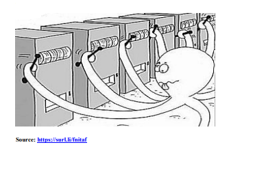
[FIGURE— slot machines cartoon (source: https://surl.li/fnitaf)]
The Multi-Armed Bandit Problem
| Meaning | A generalisation of the slot machine to multiple levers, each with a different, unknown payout probability |
| Goal | Decide which lever to pull at each step, so as to maximise total reward over time |
| Challenge | You don’t know which lever pays best without trying them. Each pull gives limited information → you must balance learning and earning |
The core dilemma: exploration vs exploitation
- Exploration — try different levers to discover their payoffs.
- Exploitation — choose the lever that seems best so far.
- Too much exploration = wasted pulls. Too little = missed better rewards.
A note on where this came from
The problem originated during World War II in sequential decision research. It was considered so difficult that scientists joked about dropping it over Germany to distract enemy researchers.
It remains a major research area — many papers at NIPS 2015 — and it is the foundation of RL: learning by trial and error, not from labelled data.
Applications today: online advertising, A/B testing, recommendation systems, clinical trials.
2. The three rules you need
Variables
| Symbol | Meaning |
|---|---|
| k | number of arms (options) |
| a ∈ {1, …, k} | an action / arm index |
| A_t | arm chosen at time t |
| R_t | reward received after pulling A_t |
| Q_t(a) | current estimate of expected reward (mean payoff) for arm a |
| N_t(a) | number of times arm a has been selected up to time t |
Rule 1 — Sample-average update
Q_{t+1}(a) ← Q_t(a) + (1 / N_t(a)) · [ R_t − Q_t(a) ]
- Moves the estimate Q_t(a) toward the newly observed reward.
- The step 1/N_t(a) is what makes it the average of all past rewards for that arm.
- Works best for stationary payoffs — means that don’t change.
Rule 2 — ε-greedy action selection
With probability 1 − ε: a = arg max_a Q_t(a) (the greedy arm)
With probability ε: pick a random arm
Balances exploitation (use the best-known arm) against exploration (try the others). Simple, and the standard baseline policy.
Rule 3 — UCB1 (Upper Confidence Bound)
A_t = arg max_a [ Q_t(a) + c · √( ln t / N_t(a) ) ]
Read the two terms separately:
- Q_t(a) — the current mean reward. This is the exploitation term.
- c · √( ln t / N_t(a) ) — the exploration bonus, larger for less-tried arms.
- c controls exploration strength.
Chooses the arm with the highest optimistic estimate. This gives directed exploration — and low regret on stationary problems.
Watch the bonus shrink (c = 2, t = 100):
| Times pulled N_t(a) | Bonus = 2·√(ln 100 / N_t(a)) |
|---|---|
| 1 | 4.2919 |
| 5 | 1.9194 |
| 10 | 1.3572 |
| 50 | 0.6070 |
| 100 | 0.4292 |
An arm pulled once carries a bonus of 4.29 — UCB will try it almost regardless of its mean. After 100 pulls the bonus is 0.43, and the mean dominates. The algorithm explores what it is uncertain about, then stops. That is the difference between UCB and ε-greedy, which keeps exploring at rate ε forever.
Summary
- Q_t(a) learns the expected payoff, by averaging rewards.
- ε-greedy gives random exploration.
- UCB gives confidence-based exploration.
Together they capture the exploration–exploitation trade-off that is central to reinforcement learning.
PART B — Adding context: the MDP
3. What changes when state arrives
A finite Markov Decision Process is the bandit problem extended, so that decisions depend not only on the action but also on the current state (context).
Purpose. To model sequential decision-making, where each action affects:
- the immediate reward, and
- the future states and their rewards.
Core idea. The agent must balance immediate versus delayed rewards to achieve optimal long-term performance.
The concrete difference:
| Bandit | MDP | |
|---|---|---|
| Estimates | one value per action → Q(a) | one value per state–action pair → q*(s, a) |
| Alternatively | — | state value assuming optimal actions → v*(s) |
Goal. Learn accurate value estimates — v*(s), q*(s, a) — in order to assign credit to actions whose outcomes occur over time.
That last phrase is the whole difficulty. In a bandit, the reward tells you immediately whether the pull was good. In an MDP, a move you make now might only pay off twenty steps later, and value functions are the bookkeeping device that traces the credit back.
4. The agent–environment interface
[FIGURE 2 — agent–environment interaction]
| # | Component | Role |
|---|---|---|
| 1 | Agent | The learner and decision-maker, selecting actions to maximise cumulative rewards over time |
| 2 | Environment | Everything external, which responds to the agent’s actions by providing new states and rewards |
| 3 | State (S_t) | The current situation or observation the agent receives from the environment at time t |
| 4 | Action (A_t) | The decision the agent makes based on the current state |
| 5 | Reward & transition | After action A_t the agent receives reward R_{t+1} and moves to a new state S_{t+1}, continuing the cycle |
The assumptions, stated plainly
- Agent and environment interact at discrete time steps: t = 0, 1, 2, …
- At step t the agent observes the state S_t ∈ 𝒮
- It produces an action A_t ∈ 𝒜(S_t)
- It gets a resulting reward R_{t+1} ∈ ℛ and a resulting next state S_{t+1}
- This is a closed loop.
Two cautions about “time step”. These are decision steps, not fractions of a second — a step is an opportunity to act, not a fixed duration. And one decision ≈ one time step. Also, 𝒮 is indexed 1 to N, and S₀ is not always literally the zeroth step.
What the action does. A_t is applied to the environment. This causes the environment’s state to change to S_{t+1}, and also produces the reward R_{t+1} — which is the result of taking A_t in state S_t and moving to S_{t+1}.
Because the next state and the reward arrive together, both are described by one joint distribution:
p(s′, r | s, a)
A physical example
[FIGURE 3 — robot arm with force and torque sensors (adapted from the Reach Robotics blog)]
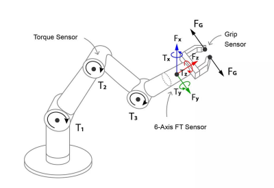
- Sensors and measurements. The arm carries torque sensors (T₁, T₂, T₃) and a 6-axis force/torque sensor measuring forces (F_x, F_y, F_z) and torques (T_x, T_y, T_z) at the end-effector, plus a grip sensor for gripping force (F_G).
- Function and feedback. These give real-time feedback on the mechanical interaction between arm and environment — load, contact pressure, orientation during movement or manipulation.
- Relevance to RL. The sensor readings define the state. The control commands (joint torques, motor inputs) are the actions. The goal — a successful grasp — is the reward. That is a complete MDP.
5. Trajectory
Run the loop and you get a chain:
S_t → A_t → R_{t+1} → S_{t+1} → A_{t+1} → R_{t+2} → S_{t+2} → A_{t+2} → …
In words: at state S_t take action A_t, get reward R_{t+1} and move to state S_{t+1}. Then take action A_{t+1}, get reward R_{t+2}, move to S_{t+2}. And so on.
This chain is called a trajectory.
[FIGURE 4 — trajectory chain, from handwritten notes]
Three things to keep straight:
- The set of states comes from 𝒮 — a discrete state space.
- The set of actions comes from 𝒜 — a discrete set of actions.
- The reward R_{t+1} is a real-valued scalar.
6. The Markov property
This is the first assumption we make, and it is what makes everything else tractable.
What is a “state”? The state at step t means whatever information is available to the agent at step t about its environment.
That can include:
- immediate sensations,
- highly processed sensations,
- and structures built up over time from sequences of sensations.
Ideally, a state should summarise past sensations so as to retain all essential information — that is, it should have the Markov property.
The definition
A state is Markov if
Pr{ S_{t+1} = s′, R_{t+1} = r | S_t, A_t, R_t, S_{t−1}, A_{t−1}, …, R_1, S_0, A_0 }
= Pr{ S_{t+1} = s′, R_{t+1} = r | S_t, A_t }
for all s′, r, and all histories.
In one sentence: the outcome is not dependent on history — the current state and action are enough to predict the system’s behaviour.
Everything struck out on the left — S_{t−1}, A_{t−1}, …, S₀, A₀ — is unnecessary. If you know where you are and what you do, the past adds nothing.
Which is why the whole model collapses to:
p(s′, r | s, a)
What can go into a state
- Agent’s position — a robot’s coordinates in a grid
- Velocity and direction — current speed and movement direction
- Sensor readings — distance to obstacles, object proximity
- Energy level — battery percentage for a drone or robot
7. The MDP tuple
An MDP M is the tuple:
M = ⟨ 𝒮, 𝒜, p, r ⟩
| Element | Type | Meaning |
|---|---|---|
| 𝒮 | finite, discrete | set of states |
| 𝒜 | finite, discrete | set of actions |
| p | 𝒮 × 𝒜 × 𝒮 → [0, 1] | probability of transition |
| r | 𝒮 × 𝒜 × 𝒮 → ℝ | expected reward |
On p. Say we are at current state s₁ and take action a₁. Then Pr(s′ | s₁, a₁) is the probability that we land in state s′. For every possible s′ we have a value; for every combination of s₁ and a₁ we have a distribution. For a large number of states, that is a large number of values — which is why the model is often the expensive part.
On r. Rather than model the whole reward distribution, we take its expected value:
r(s, a, s′) = ∫ r · Pr(r | s, a, s′) dr
Sometimes both are folded into one joint distribution: p(s′, r | s, a).
The policy
The role of the agent is to learn the policy π, which is a mapping from state to action:
π : 𝒮 × 𝒜 → [0, 1]
π(a | s) = Pr( A_t = a | S_t = s )
For every state you could have m actions, and sometimes the transition is probabilistic. The policy itself can also be deterministic:
π(a | s) = 1 for a = a₁
π(a | s) = 0 otherwise
which is often written simply as π(s) = a₁.
The agent’s goal is to maximise total expected reward. The policy that does so is called the optimal policy.
PART C — Returns: what “as much reward as possible” actually means
8. Reinforcement learning is a family, not an algorithm
Reinforcement learning is not a single algorithm. It is a family of learning methods that represent how an agent changes its policy as a result of experience.
The agent’s goal is to get as much reward as it can over the long run — that is, to maximise its returns.
Suppose the sequence of rewards after step t is R_{t+1}, R_{t+2}, R_{t+3}, …. We want to maximise the total reward, G_t, for every step t.
9. Two kinds of task
Episodic task
Interaction breaks naturally into episodes — for example, a maze game.
G_t = R_{t+1} + R_{t+2} + R_{t+3} + … + R_T
where T is the final step — the terminal state, an end to the episode.
Continuing task
There are no natural episodes; interaction goes on forever. Here we need a discounted return, with discount factor γ:
G_t = R_{t+1} + γR_{t+2} + γ²R_{t+3} + … = Σ_{k=0}^{∞} γ^k R_{t+k+1}
with 0 ≤ γ ≤ 1.
| γ | Behaviour |
|---|---|
| γ → 0 | short-sighted |
| γ → 1 | far-sighted |
γ is a controlling factor. The main intention is to maximise the expected return 𝔼[G_t] for each step t.
⚠ A point students get wrong
Is γ = 0 an immediate-reward problem? No.
Even at γ = 0 you are not solving a bandit, because the next state you will see depends on your current action. The discount controls how far ahead you value, not whether your actions have consequences. Consequences remain.
10. The recursion that everything is built on
Start from the definition and factor out one γ:
G_t = R_{t+1} + γR_{t+2} + γ²R_{t+3} + γ³R_{t+4} + …
G_t = R_{t+1} + γ[ R_{t+2} + γR_{t+3} + γ²R_{t+4} + … ]
The bracket is exactly the return starting one step later. So:
G_t = R_{t+1} + γ·G_{t+1}
Why this matters. The return at t is the current reward plus the discounted future return. Return at t starts adding from R_{t+1}; return at t+1 starts from R_{t+2}; return at t+2 from R_{t+3}. Writing it recursively links all future rewards together through a single one-step relation.
Every algorithm in Part 1 is a way of exploiting this one line. DP applies it with a known model. TD applies it to a single sampled step. Monte Carlo refuses to apply it at all and sums the whole thing.
PART D — Value functions
11. Why we need them
How do we maximise the expected return at every time step t? To carry out that maximisation we introduce the value function:
- expected future rewards
- from a start state (or state–action pair)
- following policy π
12. The state-value function
v_π(s) = 𝔼_π[ G_t | S_t = s ] = 𝔼_π[ Σ_{k=0}^{∞} γ^k R_{t+k+1} | S_t = s ], ∀ s ∈ 𝒮
What 𝔼_π means here: the expected value — the average future outcome, considering the probabilities of all possible trajectories.
How the sampling works. Starting at s, the action is sampled from the policy, A_t ~ π(·|s), and then the outcome is sampled from the dynamics, (S_{t+1}, R_{t+1}) ~ p(·, ·|S_t, A_t).
Purpose: to say which states are better under a fixed policy. It gives the long-term value of being in a state.
13. The action-value function
q_π(s, a) = 𝔼_π[ Σ_{k=0}^{∞} γ^k R_{t+k+1} | S_t = s, A_t = a ]
The one difference — and it is the whole point. In v_π, the first action is sampled from π. In q_π, the first action a is given — no sampling from π for that first step. Only afterwards is A_{t+1} ~ π(·|S_{t+1}) sampled, and the policy followed thereafter.
Purpose: from a single state, is action a₁ or action a₂ better? It exists to allow comparison among actions, and therefore to change actions.
This is why control methods learn q, not v. If you only have v_π(s), choosing an action requires a one-step lookahead through the model. If you have q_π(s, a), you just compare numbers.
14. The relationship between the two
Although these two functions are different, they have a relationship. Average the action values using the policy’s own probabilities:
v_π(s) = Σ_a π(a | s) · q_π(s, a) = 𝔼_π[ q_π(s, a) ]
(selecting the action based on policy π)
And the other direction — q in terms of v — takes one step through the dynamics and then hands over to v:
q_π(s, a) = Σ_{s′,r} p(s′, r | s, a) · [ r + γ·v_π(s′) ]
Substitute the second into the first and you have derived the Bellman expectation equation. Which is the next section.
15. The Bellman expectation equation
Start from the definition, use the recursion G_t = R_{t+1} + γG_{t+1}, and expand the expectation one step:
v_π(s) = 𝔼_π[ G_t | S_t = s ]
= 𝔼_π[ R_{t+1} + γ·G_{t+1} | S_t = s ]
= Σ_a π(a|s) Σ_{s′} Σ_r p(s′, r | s, a) · [ r + γ·𝔼_π[ G_{t+1} | S_{t+1} = s′ ] ]
v_π(s) = Σ_a π(a|s) Σ_{s′,r} p(s′, r | s, a) · [ r + γ·v_π(s′) ], ∀ s ∈ 𝒮
Reading it term by term
| Term | Meaning |
|---|---|
| π(a|s) | probability of choosing action a in state s |
| p(s′, r | s, a) | joint probability of next state s′ and reward r, given (s, a) |
| [ r + γ·v_π(s′) ] | the immediate reward plus the discounted value of the next state |
If rewards are continuous, the Σ becomes an integral.
How the expectation is actually computed
- Start at s — fixed.
- Sample a ~ π(·|s)
- Sample (s′, r) ~ p(·, ·|s, a)
- The contribution is r + γ·v_π(s′)
- Average (sum) over all possible a, s′, r
The key structural insight
Only the first step of the probabilities is explicitly expanded in the Bellman equation. The remainder of the trajectory is folded into v_π(s′).
That is the entire trick. An infinite sum over infinitely many trajectories is collapsed into one step plus a reference to a value you are also computing. Everything after step one is hidden inside the symbol v_π(s′).
Reading it on a grid
[FIGURE 5 — gridworld sketch, from handwritten notes]
Say the current state is s = 7, with two possible actions and a coin-flip policy:
π(↑ | s) = 0.5 (up)
π(→ | s) = 0.5 (right)
For “up”, the outcome is drawn from the probability distribution p(·, · | s, ↑) — we have to sample the state. The start state s is fixed; everything downstream is sampled.
16. Worked example — do it by hand
Take the two-room robot from Part 1, but now give room A a genuine choice, and follow a coin-flip policy.
Room A:
WORK→ B, reward +2 |IDLE→ stay in A, reward 0
Policy in A: π(WORK|A) = 0.5, π(IDLE|A) = 0.5
Room B:BACK→ A, reward +1 (only action)
γ = 0.5
Step 1 — write the Bellman expectation equation for each state
Room A has two actions, so we sum over both, weighted by the policy:
v_π(A) = 0.5·[ 2 + 0.5·v_π(B) ] + 0.5·[ 0 + 0.5·v_π(A) ]
Room B has one action, so the sum has one term:
v_π(B) = 1 + 0.5·v_π(A)
Step 2 — simplify the first equation
v_π(A) = 1 + 0.25·v_π(B) + 0.25·v_π(A)
Step 3 — substitute v_π(B)
v_π(A) = 1 + 0.25·(1 + 0.5·v_π(A)) + 0.25·v_π(A)
v_π(A) = 1 + 0.25 + 0.125·v_π(A) + 0.25·v_π(A)
v_π(A) = 1.25 + 0.375·v_π(A)
0.625·v_π(A) = 1.25
v_π(A) = 2.0 v_π(B) = 2.0
Step 4 — check it by iterative sweeps
Start from zero and keep applying the two equations:
| Sweep | v_π(A) | v_π(B) |
|---|---|---|
| 1 | 1.00000 | 1.00000 |
| 2 | 1.50000 | 1.50000 |
| 3 | 1.75000 | 1.75000 |
| 5 | 1.93750 | 1.93750 |
| 10 | 1.99805 | 1.99805 |
| 25 | 2.00000 | 2.00000 |
✓ Confirms the algebra.
Step 5 — now verify the v–q relationship on these numbers
Compute the action values directly:
q_π(A, WORK) = 2 + 0.5·v_π(B) = 2 + 0.5(2) = 3
q_π(A, IDLE) = 0 + 0.5·v_π(A) = 0 + 0.5(2) = 1
Now recombine them with the policy weights:
Σ_a π(a|A)·q_π(A, a) = 0.5(3) + 0.5(1) = 2 = v_π(A) ✓
And for room B, which has a single action:
q_π(B, BACK) = 1 + 0.5(2) = 2 = v_π(B) ✓
Step 6 — read what the numbers are telling you
Look at the two action values in room A: WORK = 3, IDLE = 1. The coin-flip policy is spending half its time on an action worth a third as much.
Compare against the greedy policy from Part 1:
| Policy | v(A) | v(B) |
|---|---|---|
| Coin-flip (this section) | 2.0000 | 2.0000 |
| Greedy — always WORK (Part 1) | 3.3333 | 2.6667 |
| Improvement | +1.3333 (+66.7%) | +0.6667 (+33.3%) |
And notice how you would have found that improvement. You did not need to search over policies. You evaluated the coin-flip policy, computed its action values, saw that q(A, WORK) > q(A, IDLE), and acted greedily. That single move — evaluate, then act greedily on the action values — is policy improvement, and iterating it is policy iteration.
17. Solvability: an N × N linear system
This is the point at which the theory becomes usable.
For a finite MDP with N states, the Bellman expectation equations form an N × N linear system, whose unknowns are the N value-function entries { v_π(s_i) }_{i=1}^{N}.
- N states, N unknown values: v_π(s₁), v_π(s₂), …, v_π(s_N)
- The Bellman expectation equation gives you N equations — one for each state
- Under the assumption 0 ≤ γ < 1, there is a unique solution for v_π
It converts an infinite-sum return problem into a tractable linear algebra problem.
In matrix form
Write P for the transition matrix under π and r for the vector of expected immediate rewards. Then:
v = r + γ·P·v
(I − γP)·v = rv = (I − γP)⁻¹·r
Checked on the two-room robot (greedy policy)
P = [[0, 1], [1, 0]], r = [2, 1], γ = 0.5
I − 0.5P = [[1, −0.5], [−0.5, 1]]
det(I − 0.5P) = 0.75 → non-zero, so the inverse exists and the solution is unique
v = (I − 0.5P)⁻¹·r = [3.333333, 2.666667] = [10/3, 8/3] ✓
And on the coin-flip policy
Under the coin flip, from A you go to B half the time and stay in A half the time, and the expected immediate reward in A is 0.5(2) + 0.5(0) = 1:
P = [[0.5, 0.5], [1, 0]], r = [1, 1]
v = [2.000000, 2.000000] ✓
Same answer as the hand algebra in Section 16, obtained in one matrix solve.
Why we don’t always do this. Inverting an N × N matrix costs roughly O(N³). Fine for 2 states, fine for 100. Hopeless for chess. That is precisely why the iterative and sampling methods of Part 1 exist — they trade an exact answer for an affordable one.
18. Bellman optimality
Everything above evaluates a given policy. To describe the best policy, the sum over actions becomes a max:
v*(s) = max_a Σ_{s′,r} p(s′, r | s, a) · [ r + γ·v*(s′) ]
q*(s, a) = Σ_{s′,r} p(s′, r | s, a) · [ r + γ·max_{a′} q*(s′, a′) ]
These describe the optimal value functions, assuming the best possible actions are always chosen. v* and q* define the foundation of optimal control in reinforcement learning.
The one structural difference from the expectation equations: π(a|s) has been replaced by max_a. The expectation equations are linear and can be solved by matrix inversion. The optimality equations contain a max, which makes them non-linear — no matrix inverse, which is why value iteration exists.
PART E — The first algorithm: Dynamic Programming
19. DP in RL
Dynamic Programming in reinforcement learning is a model-based approach, used when the environment’s transition dynamics p(s′, r | s, a) are fully known. It gives a systematic way to compute the optimal policy by iteratively evaluating and improving policies.
The idea:
- Start with any policy π.
- Compute its value function — policy evaluation.
- Generate a new, improved policy that acts greedily with respect to those values — policy improvement.
- Repeat until convergence.
This yields the optimal policy π* and the optimal value function v*(s).
The three equations
Policy evaluation — computes the expected value of each state under the current policy:
v_{k+1}(s) = Σ_a π(a|s) Σ_{s′,r} p(s′, r | s, a) · [ r + γ·v_k(s′) ]
Policy improvement — creates a new greedy policy that maximises expected returns:
π′(s) = arg max_a Σ_{s′,r} p(s′, r | s, a) · [ r + γ·v_π(s′) ]
Value iteration — merges both steps, approaching the optimal value function directly, without separately evaluating a full policy:
v_{k+1}(s) = max_a Σ_{s′,r} p(s′, r | s, a) · [ r + γ·v_k(s′) ]
Policy iteration is the iterative combination of evaluation and improvement. Value iteration is the faster variant that combines both in a single step.
The limitation, and why it still matters
DP assumes a perfect model and a finite state–action space, making it computationally expensive for large problems.
But it is foundational for understanding the later RL methods — Monte Carlo and Temporal-Difference learning — which approximate these same principles from experience rather than from full models.
That sentence is the bridge to Part 1. Every method there is DP with the model removed and replaced by samples.
PART F — Reference
20. Every equation on one page
| Concept | Equation |
|---|---|
| Bandit sample-average | Q_{t+1}(a) ← Q_t(a) + (1/N_t(a))[ R_t − Q_t(a) ] |
| UCB1 | A_t = arg max_a [ Q_t(a) + c·√(ln t / N_t(a)) ] |
| Markov property | Pr{S_{t+1}, R_{t+1} | S_t, A_t, …, S₀, A₀} = Pr{S_{t+1}, R_{t+1} | S_t, A_t} |
| MDP tuple | M = ⟨ 𝒮, 𝒜, p, r ⟩ |
| Policy | π(a|s) = Pr(A_t = a | S_t = s) |
| Episodic return | G_t = R_{t+1} + R_{t+2} + … + R_T |
| Discounted return | G_t = Σ_{k=0}^{∞} γ^k R_{t+k+1} |
| Return recursion | G_t = R_{t+1} + γ·G_{t+1} |
| State value | v_π(s) = 𝔼_π[ G_t | S_t = s ] |
| Action value | q_π(s,a) = 𝔼_π[ G_t | S_t = s, A_t = a ] |
| v from q | v_π(s) = Σ_a π(a|s)·q_π(s,a) |
| q from v | q_π(s,a) = Σ_{s′,r} p(s′,r|s,a)[ r + γ·v_π(s′) ] |
| Bellman expectation | v_π(s) = Σ_a π(a|s) Σ_{s′,r} p(s′,r|s,a)[ r + γ·v_π(s′) ] |
| Bellman optimality (v) | v*(s) = max_a Σ_{s′,r} p(s′,r|s,a)[ r + γ·v*(s′) ] |
| Bellman optimality (q) | q*(s,a) = Σ_{s′,r} p(s′,r|s,a)[ r + γ·max_{a′} q*(s′,a′) ] |
| Matrix solution | v = (I − γP)⁻¹·r |
| Policy evaluation | v_{k+1}(s) = Σ_a π(a|s) Σ_{s′,r} p(s′,r|s,a)[ r + γ·v_k(s′) ] |
| Policy improvement | π′(s) = arg max_a Σ_{s′,r} p(s′,r|s,a)[ r + γ·v_π(s′) ] |
| Value iteration | v_{k+1}(s) = max_a Σ_{s′,r} p(s′,r|s,a)[ r + γ·v_k(s′) ] |
21. Glossary
| Term | Meaning |
|---|---|
| State | Whatever information is available to the agent about its environment at step t |
| Markov property | The future depends only on the present state and action, not on history |
| Trajectory | The chain S_t, A_t, R_{t+1}, S_{t+1}, A_{t+1}, … |
| Episodic task | Interaction breaks naturally into episodes with a terminal state |
| Continuing task | No natural episodes; needs discounting |
| Return G_t | Total (discounted) reward from step t onward |
| Discount γ | Controls how far ahead the agent values; 0 = short-sighted, →1 = far-sighted |
| State-value v_π(s) | Expected return from s, following π — “which states are better” |
| Action-value q_π(s,a) | Expected return from s taking a first, then following π — “which action is better” |
| Bellman expectation | Value of a state = expected immediate reward + discounted value of the next state |
| Bellman optimality | Same, but taking the best action rather than averaging over the policy |
| Model-based | Uses p(s′, r | s, a) directly — e.g. DP |
22. The four things to take away
- The Markov property is what allows an entire history to collapse into p(s′, r | s, a).
- G_t = R_{t+1} + γ·G_{t+1} is the recursion every algorithm exploits.
- The Bellman equation expands only one step explicitly — the rest of the infinite future hides inside v_π(s′).
- For finite MDPs this is an N × N linear system with a unique solution. Everything in Part 1 is a way of finding that solution when N is too large to invert.
Reference: Sutton, R. S. and Barto, A. G., “Reinforcement Learning: An Introduction”, 2nd ed., MIT Press, 2018. Agent–environment interface adapted from Fig. 3.1.