🎓 Tutorial: Introduction to Machine Learning – Learning Paradigms – PAC Learning

🧠 1. What is Machine Learning?

Machine Learning (ML) is a subfield of artificial intelligence (AI) that focuses on building systems that learn from data to make decisions or predictions without being explicitly programmed.

Arthur Samuel’s definition (1959):

“Machine Learning is the field of study that gives computers the ability to learn without being explicitly programmed.”

🎯 2. Goals of Machine Learning

Discover patterns in data
Make predictions on unseen data
Improve performance with experience
Generalize well to new situations

📚 3. Learning Paradigms in ML

Machine learning problems can be broadly classified into three learning paradigms based on the supervision in training data:

✅ 3.1 Supervised Learning

Input: Labeled dataset (X, Y)
Goal: Learn a function f : X → Y to map input to output
Examples:
- Classification (e.g., spam detection)
- Regression (e.g., house price prediction)

❓ 3.2 Unsupervised Learning

Input: Unlabeled dataset (X)
Goal: Discover structure or patterns in data
Examples:
- Clustering (e.g., customer segmentation)
- Dimensionality reduction (e.g., PCA)

⚖️ 3.3 Reinforcement Learning

Input: Environment and rewards
Goal: Learn to make sequences of decisions to maximize reward
Examples:
- Game playing (e.g., AlphaGo)
- Robotics (e.g., walking, grasping)

🧪 3.4 Semi-Supervised Learning

Mix of labeled and unlabeled data
Useful when labeling is expensive

🧑‍🤝‍🧑 3.5 Self-Supervised Learning

Learns supervision signal from the data itself (e.g., predicting missing words in a sentence)

4. PAC LEARNING

Probably Approximately Correct (PAC) Learning

Source: L. G. Valiant, “A Theory of the Learnable” (1984) — @ S. S. Roy

Introduction to PAC Learning

PAC Learning, introduced by Leslie Valiant (1984), formalizes machine learning from a computational viewpoint. It asks: can a concept be learned efficiently (in polynomial time) and with high probability?

Instead of explicitly programming a machine, PAC learning treats learning as the acquisition of a recognition program from examples drawn from an unknown distribution.

The PAC Learning Framework

Instance Space: X = {0, 1}ⁿ — binary vectors of length n.
Concept (Target Function): c : X → {0, 1}.
Hypothesis Class: H, a set of candidate functions from X to {0, 1}.
Distribution D: an unknown probability distribution over X.
Training Examples: random labeled instances (x, c(x)) drawn independently and identically (i.i.d.) from D.

A learning algorithm A must, with probability at least 1 − δ, output a hypothesis h ∈ H such that:

Pr[ h(x) ≠ c(x) ] ≤ ε, where x is drawn from D.

This is what the name means: h is Probably (with confidence 1 − δ) Approximately (within error ε) Correct.

Definitions and Guarantees

PAC Learnability: a concept class C is PAC-learnable if there exists a polynomial-time algorithm such that, for any ε, δ ∈ (0, 1), the number of required training samples is polynomial in n, 1/ε, and 1/δ.

Sample Complexity (number of training examples needed):

m = O( (1/ε) · [ VCdim(H) · log(1/ε) + log(1/δ) ] )

One-sided vs. two-sided error:

One-sided: the algorithm’s hypothesis never produces a false positive.
Two-sided: errors are allowed on both positive and negative examples.

Learning Protocols

EXAMPLES routine: provides random labeled examples drawn from the distribution D.
ORACLE routine: answers, for any given instance, whether it is positive or not (a membership query).

Learnable Concept Classes

Valiant showed the following for Boolean function classes:

Class	PAC-learnable?	Notes
k-CNF expressions	Yes	Needs only the EXAMPLES routine
Monotone DNF expressions	Yes	Uses both EXAMPLES and ORACLE
General DNF	Open problem	Believed hard; no polynomial-time algorithm known
Boolean circuits	No	Unlearnable under cryptographic hardness assumptions

The Cryptographic Barrier

If certain encryption functions are computationally secure, then some Boolean functions — although computable in polynomial time — are not PAC-learnable. The striking implication: not every efficiently computable function can be efficiently learned.

VC Dimension

The VC dimension is the key measure of complexity of a hypothesis class: the size of the largest set of points the class can shatter (realize all possible labelings of). A class with finite VC dimension has finite sample complexity.

Example: linear separators (halfspaces) in ℝⁿ have VC dimension n + 1.

Criticisms and Extensions of PAC Learning

Criticisms:

Assumes noise-free data — unrealistic in practice.
Focuses on worst-case distributions.

Extensions:

Noisy PAC (tolerates label noise)
Agnostic and Bayesian variants (PAC-Bayes)
Distribution-specific PAC
Incremental / online PAC (per-example mistake bounds)

Solved Exercises

Exercise 1: Understanding the Definition

Q: Define PAC learning in your own words. What do ε and δ represent?

Solution: PAC learning means learning a function such that, with high probability (1 − δ), the learned hypothesis has error at most ε on unseen data. Here ε is the allowed error (accuracy parameter) and δ is the allowed probability of failure (confidence parameter).

Exercise 2: Sample Complexity Estimation

Q: A concept class has VC-dim = 10. Give a rough estimate of the training samples needed for PAC learning with ε = 0.05 and δ = 0.01.

Solution: Using the sample complexity formula:

m = O( (1/0.05) · [ 10 · log(20) + log(100) ] ) ≈ O( 20 · (30 + 7) ) = O(740) examples.

(Here log(20) ≈ 3.0 and log(100) ≈ 4.6 in natural log; the calculation gives an order-of-magnitude estimate, not an exact count — the constant depends on the specific bound used.)

Exercise 3: PAC Learnability Check

Q: Is the class of 3-CNF Boolean functions PAC-learnable? Justify.

Solution: Yes. 3-CNF (bounded k-CNF) is PAC-learnable using only the EXAMPLES routine: the algorithm starts with all possible clauses and deletes every clause inconsistent with an observed positive example.

Exercise 4: Importance of VC Dimension

Q: Why is VC dimension important in PAC learning?

Solution: VC dimension measures how complex a hypothesis class is. A higher VC dimension requires more examples to guarantee learning with high probability — it directly controls the sample complexity of PAC learning.

Exercise 5: One-Sided Error Property

Q: What is the advantage of one-sided error in PAC learning?

Solution: With one-sided error, the algorithm’s hypothesis never misclassifies a negative instance as positive, ensuring high precision. This matters in safety-critical systems where false positives are costly.

PAC Learning and Exercises_ML-LECTURE-1_ROY (1) (1)Download

Concept / Term	Definition / Explanation
Instance Space (𝑿)	The set of all possible input examples. In PAC learning, typically: 𝑋 = {0,1}ⁿ — all binary vectors of length n.
Concept / Target Function (𝒄)	The unknown function we aim to learn. It maps instances to labels: 𝑐 : X → {0,1}.
Hypothesis Class (𝑯)	A set of possible functions (hypotheses) that the learning algorithm can choose from: H ⊆ 2ˣ, meaning each hypothesis h ∈ H maps instances to {0,1}.
Distribution (𝑫)	An unknown probability distribution over the instance space 𝑋. The training data is drawn i.i.d. from this distribution.
Training Examples	A sequence of labeled examples drawn i.i.d. from 𝑫: (x₁, c(x₁)), …, (xₘ, c(xₘ)).
Learning Algorithm (𝑨)	The algorithm that receives training data and returns a hypothesis h ∈ H that approximates the target function c.
PAC Guarantee	The output hypothesis h satisfies: Prₓ∼𝑫[h(x) ≠ c(x)] ≤ ε with probability at least 1 − δ.
ε (epsilon)	The accuracy parameter — how close the hypothesis should be to the target function. Smaller ε means higher accuracy.
δ (delta)	The confidence parameter — how confident we want to be that the learning algorithm will return a good hypothesis.
PAC (Probably Approximately Correct)	“Probably” = with probability ≥ 1 − δ, “Approximately Correct” = error ≤ ε.
PAC Learnability	A concept class C is PAC-learnable if there exists a polynomial-time algorithm that for any ε, δ ∈ (0,1), can return a hypothesis with PAC guarantees.
Sample Complexity (𝒎)	The number of training examples needed to achieve PAC guarantees. Formula (with VC dimension): m = O(VCdim(H) ⋅ log(1/ε) + log(1/δ))
VC Dimension (VCdim(H))	The Vapnik-Chervonenkis dimension — a measure of the capacity/complexity of the hypothesis class H.
One-sided Error	Hypothesis never makes false positives (i.e., always predicts 0 for negative instances).
Two-sided Error	Errors are allowed on both positive and negative examples.

Probably Approximately Correct (PAC) learning is a foundational framework in computational learning theory, introduced by Leslie Valiant, that formalizes the concept of learnability from a theoretical, algorithmic perspective. It defines learning as the process of inferring a hypothesis that closely approximates an unknown target concept based on randomly drawn labeled examples, without relying on explicit programming. A concept class is considered PAC-learnable if a learning algorithm can, with high probability, produce a hypothesis that performs well on unseen data, using only a feasible (polynomial) number of training examples and computational steps. The framework assumes the presence of an unknown data distribution and allows the learner to receive examples either passively (as positive instances) or actively through queries to an oracle. Crucially, PAC learning emphasizes generalization: the learned hypothesis must not just fit the training data but should also perform well on new instances from the same distribution. The theory identifies specific classes of Boolean functions—such as bounded CNF and monotone DNF expressions—that are efficiently learnable, while also highlighting inherent limitations due to computational intractability and cryptographic hardness in learning more complex or unrestricted functions. Extensions to the PAC model address practical concerns like noise in data, real-valued outputs, and domain-specific biases, while the notion of VC dimension helps quantify the capacity of a hypothesis space and determine the number of examples needed for learning. Overall, PAC learning offers a rigorous, probability-based approach to understanding what can be learned, how efficiently it can be learned, and under what conditions learning is possible.

VC Dimension

🔍 Definition

The Vapnik–Chervonenkis (VC) Dimension is a fundamental measure of the capacity or expressiveness of a hypothesis class (denoted as 𝓗). It quantifies how well a model can fit various labelings of data.

💡 Key Concepts

Concept	Description
Shattering	A set of points is shattered by hypothesis class 𝓗 if 𝓗 can realize all possible labelings (2ⁿ combinations for n points).
VC Dimension	The maximum number of points that can be shattered by 𝓗. Denoted as VC(𝓗).
Intuition	Measures the ability of 𝓗 to fit any training data perfectly. Higher VC means higher complexity.
Zero Error Bound	If a hypothesis from 𝓗 achieves zero error on N examples, then N ≤ VC(𝓗).

📊 Example Interpretation

If VC(𝓗) = 3, then:
- 𝓗 can shatter any configuration of 3 points.
- It cannot shatter all configurations of 4 points.

🧠 Why It Matters

A core concept in statistical learning theory.
Helps balance model complexity vs. overfitting.
Used to understand generalization in machine learning.

📘 Historical Note

Introduced by Vladimir Vapnik and Alexey Chervonenkis.
Applicable to binary classifiers, geometric set families, and more.

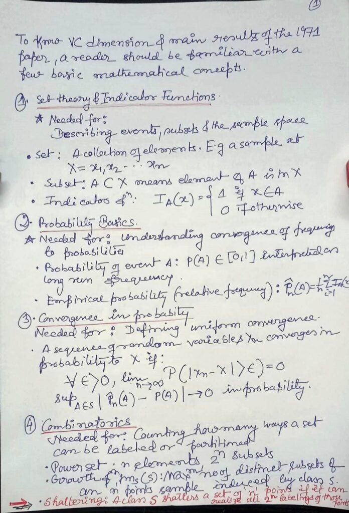
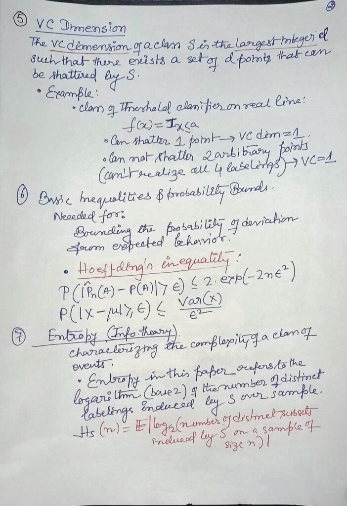
Vapnik, V. N., & Chervonenkis, A. Y. (2015). On the uniform convergence of relative frequencies of events to their probabilities. In Measures of complexity: festschrift for alexey chervonenkis (pp. 11-30). Cham: Springer International Publishing.

Vapnik–Chervonenkis Convergence: Summary

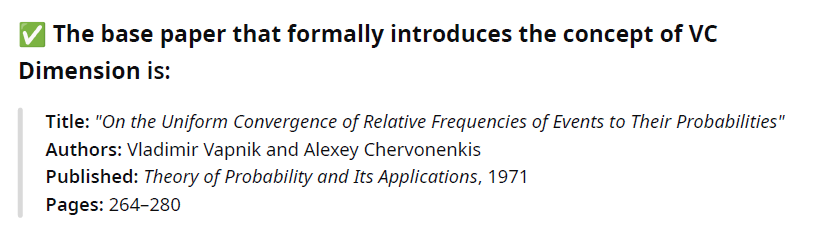
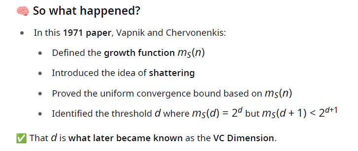
Source: V. N. Vapnik and A. Ya. Chervonenkis, “On the Uniform Convergence of Relative Frequencies of Events to Their Probabilities” (1971) — @ S. S. Roy

The Idea in Simple Words

The classical Law of Large Numbers (Bernoulli) says: for a single event A, its relative frequency in a sample converges to its true probability as the sample grows.

But machine learning needs something stronger: convergence for all events in a class S at the same time — uniform convergence — because the learner picks its hypothesis after seeing the data, from a whole class of candidates. The 1971 paper answers: under what conditions on the class S does uniform convergence hold?

Key Definitions

Term	Meaning
X	Sample space
S	A class of measurable subsets (events) of X
νₗ(A)	Relative frequency of event A ∈ S in a sample of size l
rₗ	The worst-case gap: rₗ = sup over A ∈ S of \|νₗ(A) − P(A)\|
Δˢ(x₁, …, xₗ)	Number of distinct subsets that sets in S induce on the sample x₁, …, xₗ
mˢ(l)	Growth function: the maximum of Δˢ(x₁, …, xₗ) over all samples of size l

Uniform convergence means rₗ → 0 in probability as l → ∞ — the largest gap between frequency and probability, across the entire class, vanishes.

Sufficient Condition for Uniform Convergence

If the growth function is polynomially bounded — mˢ(l) ≤ lⁿ + 1 for some finite n — then uniform convergence over S holds, with the convergence rate:

P( rₗ > ε ) ≤ 4 · mˢ(2l) · e^(−lε²/8)

The right side goes to 0 as l grows whenever mˢ grows polynomially. Under the same condition, convergence also holds almost surely.

Necessary and Sufficient Condition (the Entropy Condition)

Uniform convergence holds if and only if:

lim (l → ∞) of E[ log₂ Δˢ(x₁, …, xₗ) ] / l = 0

This quantity is the entropy of the class S — it measures the combinatorial complexity of S. If it does not vanish, uniform convergence fails.

Growth Function Examples

Class S	Growth function mˢ(l)
Rays {x ≤ a} on ℝ	l + 1
Half-spaces in ℝⁿ	Φ(n, l) ≤ lⁿ + 1
Open sets on [0, 1]	2ˡ (always shatters — no uniform convergence)

Sample Size Estimation

To guarantee P( sup over A ∈ S of |νₗ(A) − P(A)| > ε ) ≤ δ, it suffices to take:

l ≥ (16/ε²) · ( n · log(2/ε) + log(1/δ) )

where n is the polynomial degree bounding the growth function.

The VC Dimension (as it appears in the 1971 paper)

The paper never uses the name “VC dimension,” but the concept is fully there, through shattering:

Term	Description
Shattering	S shatters a sample of size l if mˢ(l) = 2ˡ — every possible labeling of the sample is induced by some set in S
VC dimension d	The largest l for which mˢ(l) = 2ˡ. If shattering holds at l = d but fails at l = d + 1, then VC(S) = d

The key theorem of the paper: the growth function mˢ(r) is either identically equal to 2ʳ, or else it is majorized by a power function rⁿ + 1, where n is the first value of r at which mˢ(r) < 2ʳ. In other words — a class either shatters everything forever, or its growth function collapses from exponential to polynomial exactly at its VC dimension. There is no middle behavior.

Translation Table: 1971 Paper → Modern Terminology

Concept	Paper’s notation	Modern term
Class of events S	S	Hypothesis class H
Δˢ(x₁, …, xₗ)	Subsample induction count	Number of dichotomies on a sample
mˢ(l)	Growth function	Shattering / growth function
First r where mˢ(r) < 2ʳ	—	VC dimension (+1 relationship: d = that r minus 1)

VC Dimension Examples

Class	VC Dimension
Rays {x ≤ a} on ℝ	1
Half-spaces in ℝⁿ	n + 1
Open subsets of [0, 1]	Infinite (mˢ(l) = 2ˡ for all l)

Why It Matters

VC dimension quantifies the capacity (complexity) of a hypothesis class.
Finite VC dimension implies uniform convergence of empirical frequencies to true probabilities — which means empirical error is a trustworthy estimate of true error.
This became the core criterion for learnability in statistical learning theory, and the direct foundation of the sample-complexity results in PAC learning.

convergence Summary (1)Download

Download some solved problem on VC Dimension

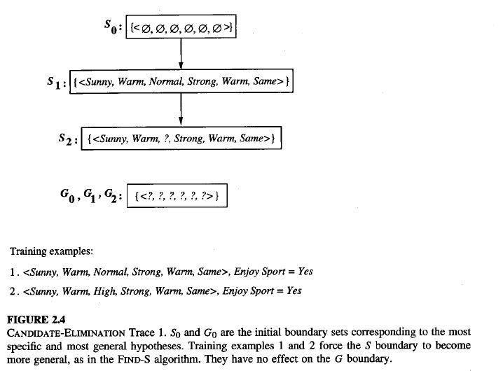
4 VC Dimension questionsROY Download

FIND-S: FINDING A MAXIMALLY SPECIFIC HYPOTHESIS

(Ref : Mitchell, T. M. (1997). Machine Learning. McGraw-Hill.)

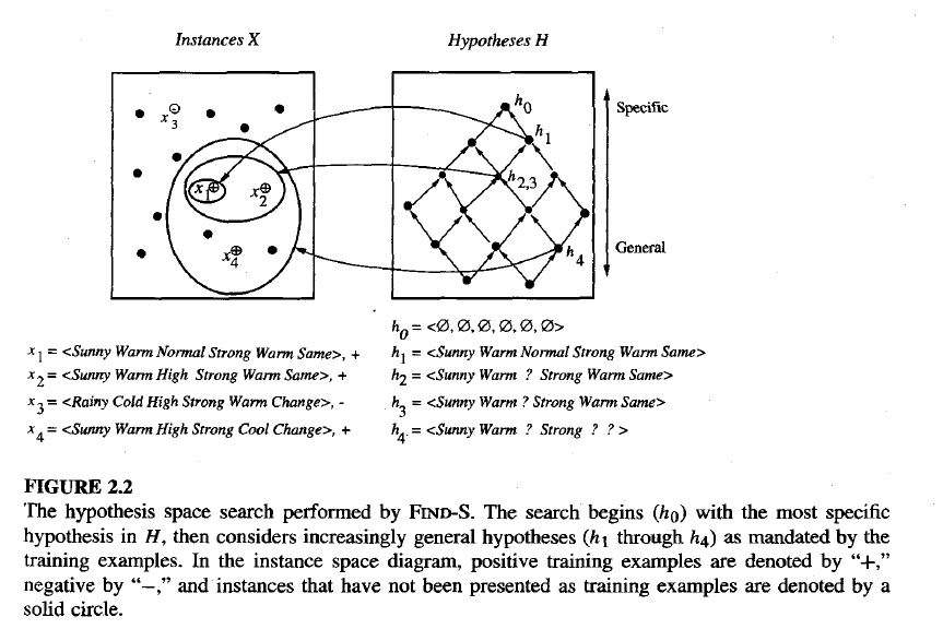
Find-S algorithm tutorial-SSROY (1)Download

A Systematic Approach to Learning with the Candidate Elimination Algorithm

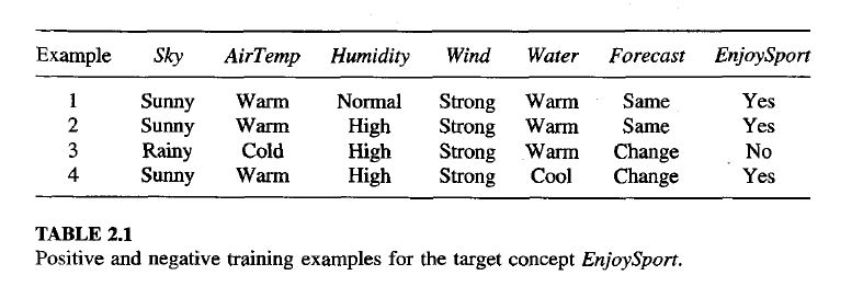
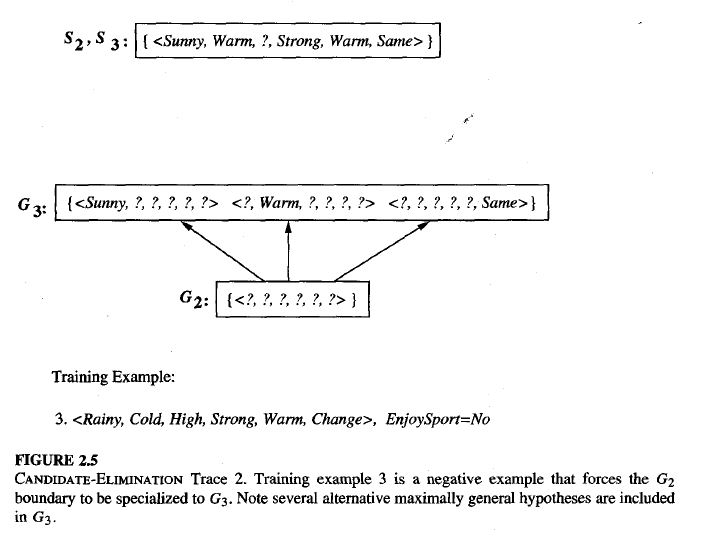
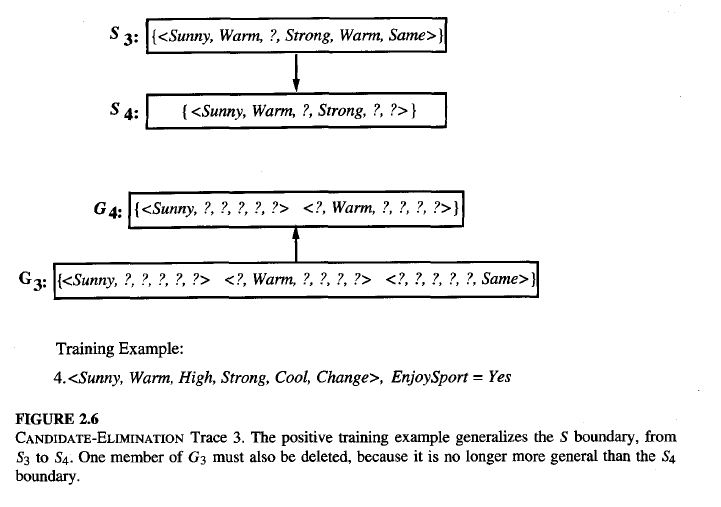
Candidate Elimination Algorithm

Candidate elimination tutorial-1SSROY (1)Download

Revisit again : Candidate Elimination Algorithm — Simple Steps

Step 1 – Initialization

S = most specific hypothesis (matches nothing yet)
G = most general hypothesis (matches everything)

Step 2 – Process each training example:

When the example is Positive (Yes)

Adjust S so it becomes just general enough to include this example.
Remove from G any hypothesis that does not include this example.

When the example is Negative (No)

Remove from S any hypothesis that still includes this example.
Specialize each hypothesis in G that includes this example, just enough to exclude it, while still including all positive examples so far.
Remove any hypotheses from G that are more specific than others or duplicate.

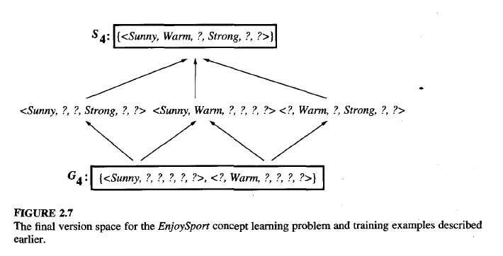
Step 3 – Completion

After all examples are processed, the version space is the set of hypotheses between S and G.
S represents the narrowest possible rule consistent with the data.
G represents the broadest possible rule consistent with the data.