K-MEANS CLUSTERING
K-Means clustering is a powerful and efficient algorithm for grouping data points into clusters based on similarity. Despite its simplicity, it is widely used in various fields due to its scalability, ease of use, and effectiveness in uncovering patterns in large datasets. However, it is important to consider its limitations, such as sensitivity to initialization and the need for a predefined number of clusters. Despite these challenges, K-Means remains one of the most popular clustering algorithms in data analysis and machine learning.
Implement the K-Means algorithm with K = 2 on the data points (185, 72), (170, 56), (168, 60), (179, 68), (182, 72), and (188, 77) for two iterations, and display the resulting clusters. Initially, select the first two data points as the initial centroids.
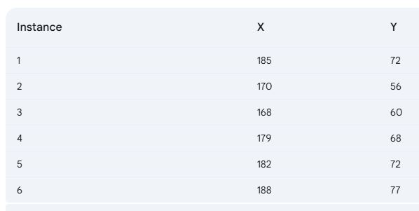
In the initial step, we determine the similarity between data points using the Euclidean distance metric.
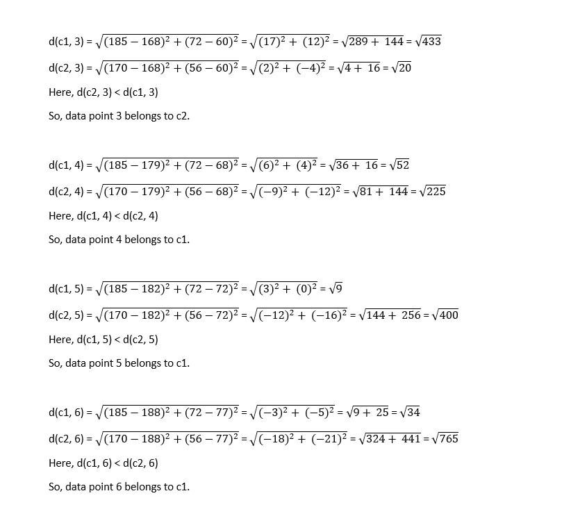
In tabular-form it can be represented as,
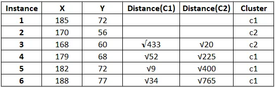
The result after first iteration.

In the second iteration, calculating centroids again,

Calculating distances again,
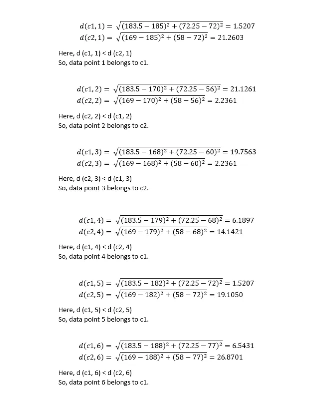
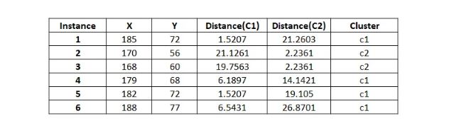
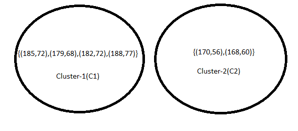
As two iterations have already been completed as required by the problem, the numerical process concludes here. Since the clustering remains unchanged after the second iteration, the process will be terminated, even if the question does not explicitly state to do so.
Read more: Unsupervised learningK-MODES CLUSTERING
K-Modes Clustering — Theory and a Fully Worked Example
~S S Roy
Theory (the minimum you need)
What it is. K-Modes is the categorical-data counterpart of k-means. K-means fails on categorical data because means and Euclidean distance are meaningless for labels like “Red” or “Cotton”. K-Modes replaces:
- Means → Modes (the most frequent category per feature in a cluster)
- Euclidean distance → Simple matching dissimilarity (count of mismatched features)
Dissimilarity. For two categorical vectors x = (x₁, …, xₚ) and y = (y₁, …, yₚ):
d(x, y) = Σⱼ 1{xⱼ ≠ yⱼ} (the number of features where the two records disagree; 0 = identical, p = completely different)
Cluster representative (mode). For each cluster and each feature, take the most frequent category in that cluster. The vector of these per-feature modes is the cluster center m = (m₁, …, mₚ).
Objective. K-Modes minimizes the total within-cluster mismatches:
Cost(C₁, …, Cₖ) = Σᵢ d(xᵢ, mode of its cluster)
Algorithm (Huang, 1998).
- Initialize k modes (random rows, or Huang/Cao seeding).
- Assign each record to the nearest mode by simple matching dissimilarity.
- Update each cluster’s mode: per feature, take the most frequent category (break ties by a fixed rule).
- Repeat assign ↔ update until the modes stop changing.
Each iteration costs O(nkp) for n rows, k clusters, p features — fast for typical categorical tables.
Choosing k. Run for k = 1, 2, … and use the elbow of the cost curve, held-out assignment cost, or stability across random seeds. For mixed numeric + categorical data, use k-prototypes instead.
K-Modes Worked Example with Multiple Iterations
We’ll use the toy dataset:
| ID | Size | Fit | Color | Fabric |
|---|---|---|---|---|
| 1 | S | Slim | Red | Cotton |
| 2 | S | Slim | Blue | Cotton |
| 3 | M | Regular | Blue | Cotton |
| 4 | L | Regular | Blue | Polyester |
| 5 | L | Regular | Green | Polyester |
| 6 | M | Slim | Red | Cotton |
| 7 | M | Regular | Blue | Polyester |
| 8 | L | Regular | Blue | Cotton |
We’ll set k = 2 clusters.
Step 1. Initialization (choose 2 random seeds)
Let’s pick:
- Mode₁ (initial) ← Row 2 = (S, Slim, Blue, Cotton)
- Mode₂ (initial) ← Row 5 = (L, Regular, Green, Polyester)
These are less “clean,” so convergence takes longer.
Step 2. First Assignment
Compute mismatches for each row vs each mode:
| ID | Row (Size, Fit, Color, Fabric) | d to Mode₁ (S,Slim,Blue,Cotton) | d to Mode₂ (L,Regular,Green,Poly) | Assign |
|---|---|---|---|---|
| 1 | (S,Slim,Red,Cotton) | 1 (Color) | 4 | C₁ |
| 2 | (S,Slim,Blue,Cotton) | 0 | 4 | C₁ |
| 3 | (M,Reg,Blue,Cotton) | 2 (Size,Fit) | 2 (Size,Fabric) | C₁ (tie→C₁) |
| 4 | (L,Reg,Blue,Poly) | 2 (Size,Fabric) | 1 (Color) | C₂ |
| 5 | (L,Reg,Green,Poly) | 3 | 0 | C₂ |
| 6 | (M,Slim,Red,Cotton) | 2 (Size,Color) | 4 | C₁ |
| 7 | (M,Reg,Blue,Poly) | 2 (Size,Fabric) | 1 (Color) | C₂ |
| 8 | (L,Reg,Blue,Cotton) | 2 (Size,Fabric) | 1 (Color) | C₂ |
Clusters after Iteration 1:
- C₁ = {1,2,3,6}
- C₂ = {4,5,7,8}
Step 3. Update Modes
Mode₁ (C₁ rows 1,2,3,6):
- Size: S(2), M(2) → tie → pick S (tie-break fixed order)
- Fit: Slim(3), Reg(1) → Slim
- Color: Red(2), Blue(2) → tie → pick Blue
- Fabric: Cotton(4) → Cotton
→ Mode₁′ = (S, Slim, Blue, Cotton)
Mode₂ (C₂ rows 4,5,7,8):
- Size: L(3), M(1) → L
- Fit: Reg(4) → Regular
- Color: Blue(3), Green(1) → Blue
- Fabric: Polyester(2), Cotton(2) → tie → pick Polyester
→ Mode₂′ = (L, Regular, Blue, Polyester)
Step 4. Second Assignment
Now compare all rows again vs updated modes:
| ID | Row | d to Mode₁′ (S,Slim,Blue,Cotton) | d to Mode₂′ (L,Reg,Blue,Poly) | Assign |
|---|---|---|---|---|
| 1 | (S,Slim,Red,Cotton) | 1 (Color) | 3 (Size,Fit,Fabric) | C₁ |
| 2 | (S,Slim,Blue,Cotton) | 0 | 3 (Size,Fit,Fabric) | C₁ |
| 3 | (M,Reg,Blue,Cotton) | 2 (Size,Fit) | 1 (Fabric) | C₂ |
| 4 | (L,Reg,Blue,Poly) | 3 (Size,Fit,Fabric) | 0 | C₂ |
| 5 | (L,Reg,Green,Poly) | 4 | 1 (Color) | C₂ |
| 6 | (M,Slim,Red,Cotton) | 2 (Size,Color) | 3 (Size,Fabric,Color) | C₁ |
| 7 | (M,Reg,Blue,Poly) | 3 (Size,Fit,Fabric) | 1 (Size) | C₂ |
| 8 | (L,Reg,Blue,Cotton) | 2 (Size,Fit) | 1 (Fabric) | C₂ |
Clusters after Iteration 2:
- C₁ = {1,2,6}
- C₂ = {3,4,5,7,8}
Step 5. Update Modes Again
Mode₁ (rows 1,2,6):
- Size: S(2), M(1) → S
- Fit: Slim(3) → Slim
- Color: Red(2), Blue(1) → Red
- Fabric: Cotton(3) → Cotton
→ Mode₁″ = (S, Slim, Red, Cotton)
Mode₂ (rows 3,4,5,7,8):
- Size: L(3), M(2) → L
- Fit: Reg(5) → Regular
- Color: Blue(4), Green(1) → Blue
- Fabric: Polyester(3), Cotton(2) → Polyester
→ Mode₂″ = (L, Regular, Blue, Polyester)
Step 6. Third Assignment
Check again with new Mode₁″ and Mode₂″:
| ID | Row | d to Mode₁″ (S,Slim,Red,Cotton) | d to Mode₂″ (L,Reg,Blue,Poly) | Assign |
|---|---|---|---|---|
| 1 | (S,Slim,Red,Cotton) | 0 | 4 | C₁ |
| 2 | (S,Slim,Blue,Cotton) | 1 (Color) | 3 (Size,Fit,Fabric) | C₁ |
| 3 | (M,Reg,Blue,Cotton) | 3 (Size,Fit,Color) | 1 (Fabric) | C₂ |
| 4 | (L,Reg,Blue,Poly) | 4 | 0 | C₂ |
| 5 | (L,Reg,Green,Poly) | 3 | 1 (Color) | C₂ |
| 6 | (M,Slim,Red,Cotton) | 1 (Size) | 4 | C₁ |
| 7 | (M,Reg,Blue,Poly) | 4 | 1 (Size) | C₂ |
| 8 | (L,Reg,Blue,Cotton) | 3 (Size,Fit,Color) | 1 (Fabric) | C₂ |
Clusters after Iteration 3:
- C₁ = {1,2,6}
- C₂ = {3,4,5,7,8}
Step 7. Update Modes
- Mode₁ stays (S, Slim, Red, Cotton)
- Mode₂ stays (L, Regular, Blue, Polyester)
→ No change → algorithm converged after 3 iterations.
Final Results
Final modes (cluster representatives):
- Cluster 1 → (S, Slim, Red, Cotton)
- Cluster 2 → (L, Regular, Blue, Polyester)
Cluster memberships:
- C₁ = {1,2,6}
- C₂ = {3,4,5,7,8}
Total cost:
- C₁ mismatches = 0 + 1 + 1 = 2
- C₂ mismatches = 1 + 0 + 1 + 1 + 1 = 4
- Total = 6 mismatches
Further reading
- Z. Huang (1998). “Extensions to the k-means algorithm for clustering large data sets with categorical values.” Data Mining and Knowledge Discovery.
- Z. Huang (1997). “Clustering large data sets with mixed numeric and categorical values.” Proceedings of the 1st Pacific-Asia Conference on KDD (k-prototypes).
Hierarchical Clustering
Hierarchical Clustering — A Short Tutorial with a Worked Example
~S S Roy
Theory (the minimum you need)
What it is. Hierarchical clustering builds a tree of clusters (a dendrogram) instead of a single flat partition. You do not need to fix the number of clusters k in advance — you cut the tree afterwards at any level to get as many clusters as you want.
Two directions:
- Agglomerative (bottom-up): start with every point as its own cluster; repeatedly merge the two closest clusters until one cluster remains. This is the standard method and the one used below.
- Divisive (top-down): start with all points in one cluster and recursively split. Rarely used in practice because splitting is computationally harder.
Linkage — how do we measure distance between two clusters? Given a distance d(x, y) between points (usually Euclidean), the distance between clusters A and B can be defined as:
- Single linkage: min distance between any point in A and any point in B. Finds elongated, chain-like clusters; sensitive to noise (“chaining effect”).
- Complete linkage: max distance between any point in A and any point in B. Produces compact, roughly equal-sized clusters.
- Average linkage: average of all pairwise distances between A and B. A compromise between the two.
- Ward’s method: merge the pair whose union gives the smallest increase in total within-cluster variance. Often the best default for numeric data.
Algorithm (agglomerative).
- Compute the n × n pairwise distance matrix.
- Merge the two clusters with the smallest linkage distance.
- Update the distance matrix (recompute distances from the new merged cluster to all others using the chosen linkage).
- Repeat steps 2–3 until a single cluster remains. Record the height (distance) of every merge — this gives the dendrogram.
Complexity. Naïve implementation is O(n³); with priority queues it is O(n² log n), and memory is O(n²) for the distance matrix. This is why hierarchical clustering suits small-to-medium datasets (thousands of points), not millions.
Worked Example (Single Linkage, Step by Step)
Take five one-dimensional points (1-D keeps the arithmetic exact; the procedure is identical in any dimension):
| Point | A | B | C | D | E |
|---|---|---|---|---|---|
| Value | 1 | 2 | 4 | 7 | 8 |
Distance = absolute difference. Initial distance matrix:
| A | B | C | D | E | |
|---|---|---|---|---|---|
| A | 0 | 1 | 3 | 6 | 7 |
| B | 1 | 0 | 2 | 5 | 6 |
| C | 3 | 2 | 0 | 3 | 4 |
| D | 6 | 5 | 3 | 0 | 1 |
| E | 7 | 6 | 4 | 1 | 0 |
Step 1 — Merge the closest pair
Smallest distance is 1, achieved by both (A, B) and (D, E) — a tie. Break ties in a fixed order (first pair found): merge A and B at height 1.
Clusters: {A,B}, {C}, {D}, {E}.
Update distances from {A,B} using single linkage (minimum):
- d({A,B}, C) = min(3, 2) = 2
- d({A,B}, D) = min(6, 5) = 5
- d({A,B}, E) = min(7, 6) = 6
| {A,B} | C | D | E | |
|---|---|---|---|---|
| {A,B} | 0 | 2 | 5 | 6 |
| C | 2 | 0 | 3 | 4 |
| D | 5 | 3 | 0 | 1 |
| E | 6 | 4 | 1 | 0 |
Step 2 — Merge the next closest pair
Smallest distance is 1: merge D and E at height 1.
Clusters: {A,B}, {C}, {D,E}.
- d({A,B}, {D,E}) = min(5, 6) = 5
- d(C, {D,E}) = min(3, 4) = 3
| {A,B} | C | {D,E} | |
|---|---|---|---|
| {A,B} | 0 | 2 | 5 |
| C | 2 | 0 | 3 |
| {D,E} | 5 | 3 | 0 |
Step 3 — Merge again
Smallest distance is 2: merge {A,B} and C at height 2.
Clusters: {A,B,C}, {D,E}.
- d({A,B,C}, {D,E}) = min(5, 3) = 3
Step 4 — Final merge
Merge {A,B,C} and {D,E} at height 3. One cluster remains — done.
The dendrogram
The recorded merge heights (1, 1, 2, 3) define the tree:
height 3  ────────────┬────────────
                      │
height 2  ──────┬─────│────────────
                │     │
height 1  ─┬────│─────│──────┬─────
           │    │     │      │
           A─B  C     │      D─E
           └─┬──┘     │
             └────────┴──────┘
Cutting the dendrogram gives the flat clustering:
- Cut at height 2.5 → 2 clusters: {A, B, C} and {D, E}
- Cut at height 1.5 → 3 clusters: {A, B}, {C}, {D, E}
The largest vertical gap between successive merge heights (here between 1 and 2, or 2 and 3) is a common heuristic for where to cut.
Note on linkage choice: with complete linkage the updates would use max instead of min — e.g., d({A,B}, C) = max(3, 2) = 3 — and the merge order and heights can change. On this small dataset the final 2-cluster partition happens to be the same; on real data the choice of linkage often changes the result substantially.
Minimal Python (SciPy)
import numpy as np
from scipy.cluster.hierarchy import linkage, dendrogram, fcluster
import matplotlib.pyplot as plt

X = np.array([[1], [2], [4], [7], [8]])   # points A..E

Z = linkage(X, method='single')            # try 'complete', 'average', 'ward'
print(Z)                                   # each row: cluster i, cluster j, height, size

dendrogram(Z, labels=['A', 'B', 'C', 'D', 'E'])
plt.ylabel('Merge distance')
plt.show()

labels = fcluster(Z, t=2.5, criterion='distance')   # cut at height 2.5
print(labels)                              # → [1 1 1 2 2]  i.e. {A,B,C} and {D,E}
When to use it (and when not)
- Use it when you want the full cluster hierarchy, when k is unknown, when the dataset is small enough for an n × n distance matrix, or when a dendrogram itself is the deliverable (taxonomy, phylogenetics, document organization).
- Avoid it for very large datasets (memory and time scale quadratically), and remember merges are greedy and irreversible — a bad early merge can never be undone, unlike k-means which re-assigns points every iteration.
Aggiomerative Hierarchical Clustering(Single LInk)
A dendrogram is a tree diagram that records the complete history of agglomerative hierarchical clustering: each data point starts at the bottom as its own cluster, and at every step the two closest clusters are merged, with the height of the joining bar showing the distance at which that merge occurred. In this example, using single-link (minimum distance) on the dataset {12, 17, 18, 24, 50, 52}, the points 17 and 18 join first at distance 1, then 50 and 52 at distance 2, after which 12 joins {17, 18} at 5 and 24 joins them at 6 — building two compact groups, {12, 17, 18, 24} and {50, 52}. The final merge of these two groups happens only at distance 26, and this large jump from 6 to 26 is the key insight the dendrogram gives us: cutting the tree anywhere in that gap yields the natural clustering of the data into two well-separated clusters.
DBSCAN
~S S Roy
Very short theory
DBSCAN (Density-Based Spatial Clustering of Applications with Noise) groups together points that are closely packed and marks points lying alone in low-density regions as noise (outliers). Unlike k-means, it needs no k, finds arbitrarily shaped clusters, and detects outliers automatically. It uses two parameters:
- ε (epsilon): the maximum distance for two points to be considered neighbors.
- MinPts: the minimum number of points (including the point itself) in an ε-neighborhood to make a point dense.
Every point gets one of three labels:
- Core point: has at least MinPts points (including itself) within ε.
- Border point: has fewer than MinPts within ε, but lies within ε of a core point.
- Noise point: neither core nor border.
How clusters form: pick an unvisited core point, start a cluster, and expand it through every core point within ε of a core point already in the cluster; border points join the cluster of a nearby core but cannot expand it further. Expansion happens only through core points — this rule decides the final clusters.
Worked example (12 points, ε = 1.9, MinPts = 4)
We have 12 points P1–P12. The pairwise Euclidean distances, Distance(Pᵢ, Pⱼ) = √((Xⱼ−Xᵢ)² + (Yⱼ−Yᵢ)²), give this matrix. For example, for P1 (4.5, 8) and P2 (5, 7): √(0.5² + (−1)²) = √1.25 ≈ 1.12.
| P1 | P2 | P3 | P4 | P5 | P6 | P7 | P8 | P9 | P10 | P11 | P12 | |
|---|---|---|---|---|---|---|---|---|---|---|---|---|
| P1 | 0.00 | 1.12 | 2.12 | 3.91 | 6.02 | 5.59 | 5.70 | 5.41 | 4.03 | 1.58 | 2.06 | 3.16 |
| P2 | 1.12 | 0.00 | 1.12 | 2.83 | 5.00 | 4.47 | 4.61 | 4.47 | 3.16 | 2.06 | 1.41 | 2.50 |
| P3 | 2.12 | 1.12 | 0.00 | 1.80 | 3.91 | 3.64 | 3.61 | 3.35 | 3.20 | 3.16 | 2.06 | 2.92 |
| P4 | 3.91 | 2.83 | 1.80 | 0.00 | 2.24 | 2.00 | 1.80 | 2.00 | 3.16 | 4.72 | 3.16 | 3.50 |
| P5 | 6.02 | 5.00 | 3.91 | 2.24 | 0.00 | 2.24 | 1.12 | 1.00 | 5.00 | 6.95 | 5.39 | 5.59 |
| P6 | 5.59 | 4.47 | 3.64 | 2.00 | 2.24 | 0.00 | 1.12 | 2.83 | 3.16 | 6.02 | 4.24 | 4.03 |
| P7 | 5.70 | 4.61 | 3.61 | 1.80 | 1.12 | 1.12 | 0.00 | 1.80 | 4.03 | 6.40 | 4.72 | 4.74 |
| P8 | 5.41 | 4.47 | 3.35 | 2.00 | 1.00 | 2.83 | 1.80 | 0.00 | 5.10 | 6.50 | 5.10 | 5.50 |
| P9 | 4.03 | 3.16 | 3.20 | 3.16 | 5.00 | 3.16 | 4.03 | 5.10 | 0.00 | 3.64 | 2.00 | 1.12 |
| P10 | 1.58 | 2.06 | 3.16 | 4.72 | 6.95 | 6.02 | 6.40 | 6.50 | 3.64 | 0.00 | 1.80 | 2.55 |
| P11 | 2.06 | 1.41 | 2.06 | 3.16 | 5.39 | 4.24 | 4.72 | 5.10 | 2.00 | 1.80 | 0.00 | 1.12 |
| P12 | 3.16 | 2.50 | 2.92 | 3.50 | 5.59 | 4.03 | 4.74 | 5.50 | 1.12 | 2.55 | 1.12 | 0.00 |
Step 1: Find each point’s ε-neighbors and classify
Read each row of the matrix and keep the entries ≤ 1.9. Count includes the point itself; core requires count ≥ 4.
| Point | Neighbors within ε = 1.9 | Count (incl. self) | Core? |
|---|---|---|---|
| P1 | P2 (1.12), P10 (1.58) | 3 | No |
| P2 | P1 (1.12), P3 (1.12), P11 (1.41) | 4 | Yes |
| P3 | P2 (1.12), P4 (1.80) | 3 | No |
| P4 | P3 (1.80), P7 (1.80) | 3 | No |
| P5 | P7 (1.12), P8 (1.00) | 3 | No |
| P6 | P7 (1.12) | 2 | No |
| P7 | P4 (1.80), P5 (1.12), P6 (1.12), P8 (1.80) | 5 | Yes |
| P8 | P5 (1.00), P7 (1.80) | 3 | No |
| P9 | P12 (1.12) | 2 | No |
| P10 | P1 (1.58), P11 (1.80) | 3 | No |
| P11 | P2 (1.41), P10 (1.80), P12 (1.12) | 4 | Yes |
| P12 | P9 (1.12), P11 (1.12) | 3 | No |
Core points: P2, P7, P11. All other points are border or noise, decided next.
Step 2: Connect the core points
- d(P2, P11) = 1.41 ≤ ε → P2 and P11 are directly density-reachable → same cluster.
- d(P7, P2) = 4.61 and d(P7, P11) = 4.72, both > ε → P7 is not connected to them → separate cluster.
So there are two clusters: one built on cores {P2, P11}, one built on core {P7}.
Step 3: Attach border points, mark noise
Each non-core point joins a cluster only if it is within ε of a core point:
- P1 → within ε of core P2 → border, Cluster 1
- P3 → within ε of core P2 → border, Cluster 1
- P10 → within ε of core P11 → border, Cluster 1
- P12 → within ε of core P11 → border, Cluster 1
- P4 → within ε of core P7 → border, Cluster 2
- P5 → within ε of core P7 → border, Cluster 2
- P6 → within ε of core P7 → border, Cluster 2
- P8 → within ε of core P7 → border, Cluster 2
- P9 → its only neighbor is P12, which is a border point, not core. Border points cannot recruit new members. → Noise
Final result
| Cluster | Core points | Border points | Members |
|---|---|---|---|
| Cluster 1 | P2, P11 | P1, P3, P10, P12 | P1, P2, P3, P10, P11, P12 |
| Cluster 2 | P7 | P4, P5, P6, P8 | P4, P5, P6, P7, P8 |
| Noise | — | — | P9 |
Key takeaway: DBSCAN finds the dense regions and grows clusters only through core points. P9 illustrates the noise rule perfectly — it touches the cluster (via border point P12) but no core point, so it stays an outlier. This is exactly the behavior k-means cannot give you: automatic outlier detection with no k specified in advance.
Expectation-Maximization (EM) Algorithm
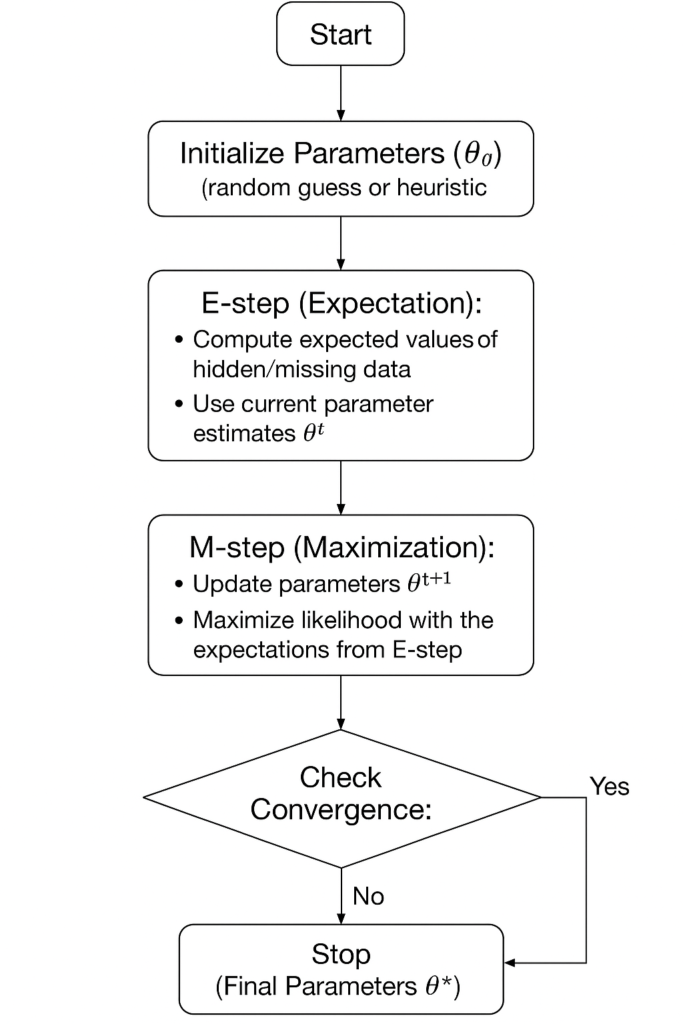
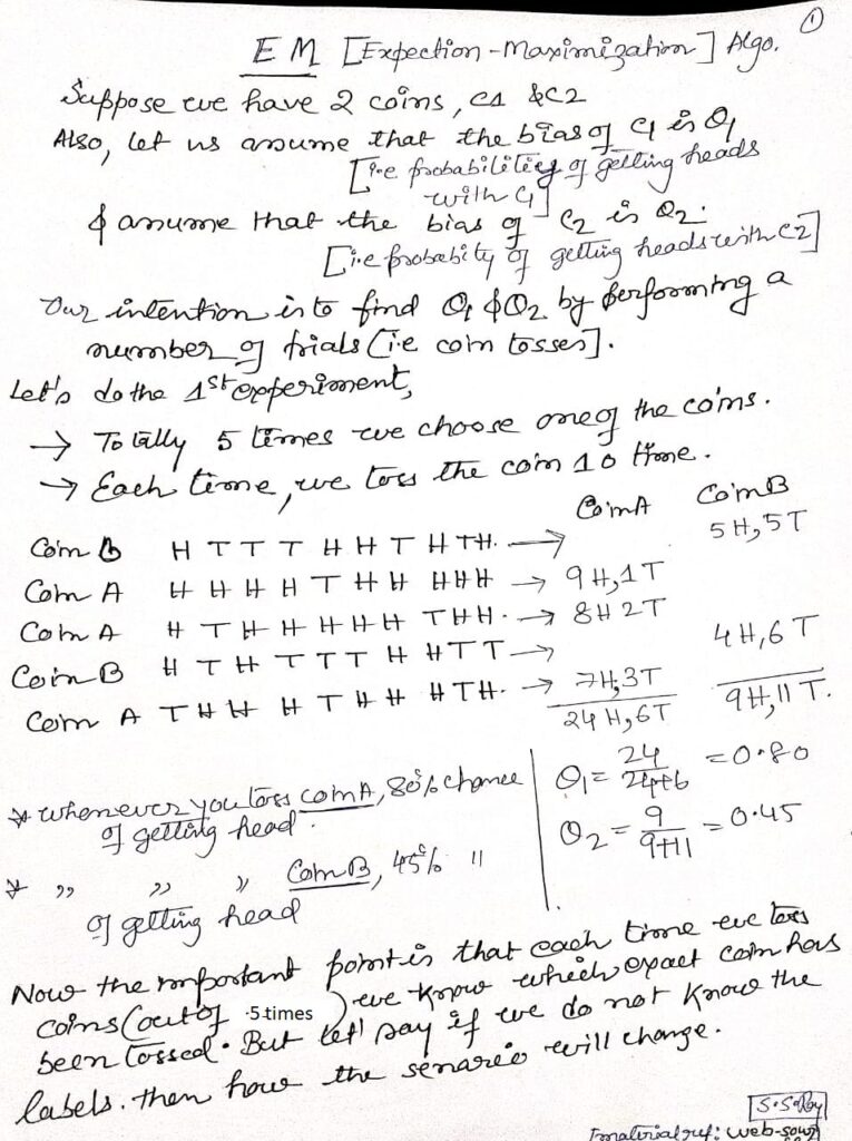
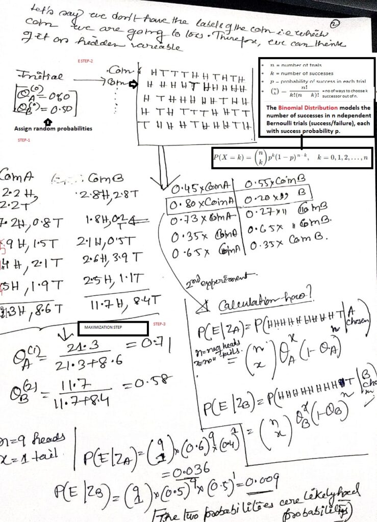
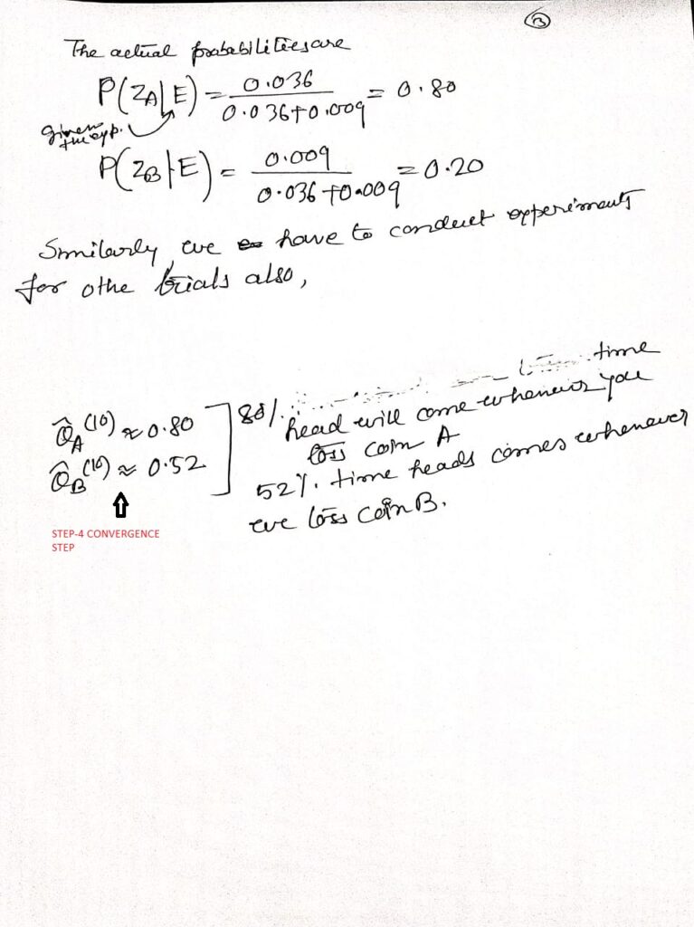
The Expectation-Maximization (EM) algorithm is a powerful iterative method to estimate parameters of probabilistic models when data is incomplete, uncertain, or involves hidden variables.
- Idea: Direct maximization of likelihood is hard due to missing/hidden data. EM solves this by alternating between two intuitive steps:
- E-step (Expectation): Compute the expected value of hidden variables using current parameters.
- M-step (Maximization): Update parameters by maximizing the likelihood with these expectations.
This repeat–refine process guarantees non-decreasing likelihood and converges to a local optimum. EM underlies key methods like Gaussian Mixture Models, Hidden Markov Models, and clustering with incomplete data, making it a cornerstone of statistical learning.
Other applications : Image Processing: Segmentation, denoising;Missing Data Problems: Robust parameter estimation;Anomaly Detection: Fraud, outliers.,Medical & Bioinformatics: Gene expression, disease models;Recommender Systems: Latent factor models.
Mathematical Prerequisites:

MCQs on EM
- What is the main purpose of the EM algorithm?
A) Solve linear equations
B) Maximize likelihood with incomplete data
C) Minimize squared error
D) Perform gradient descent
Answer: B) Maximize likelihood with incomplete data - Which two main steps does EM consist of?
A) Encode and Decode
B) Expectation and Maximization
C) Sampling and Updating
D) Forward and Backward
Answer: B) Expectation and Maximization - EM is typically used when:
A) All data is observed
B) Data is incomplete or has latent variables
C) The dataset is small
D) The data is categorical only
Answer: B) Data is incomplete or has latent variables - The EM algorithm guarantees:
A) Convergence to global maximum likelihood
B) Convergence to a local maximum of likelihood
C) Exact posterior distributions
D) Linear convergence speed
Answer: B) Convergence to a local maximum of likelihood
- In the Gaussian Mixture Model (GMM), what does the E-step compute?
A) Update the means of clusters
B) Update the covariance matrices
C) Compute responsibilities (probabilities of points belonging to clusters)
D) Compute the gradient of the likelihood
Answer: C) Compute responsibilities (probabilities of points belonging to clusters) - Which of the following is a limitation of EM?
A) Requires derivative computations
B) Sensitive to initial parameter values
C) Can only handle two clusters
D) Works only with discrete data
Answer: B) Sensitive to initial parameter values - After how many iterations does EM converge?
A) Always in one iteration
B) Depends on the convergence criterion (e.g., change in likelihood)
C) Always after 10 iterations
D) EM never converges
Answer: B) Depends on the convergence criterion (e.g., change in likelihood) - Which of these is true about the log-likelihood in EM?
A) It decreases in each iteration
B) It increases or stays the same in each iteration
C) It oscillates randomly
D) It remains constant
Answer: B) It increases or stays the same in each iteration
- Consider EM applied to a mixture of two Gaussians with identical variances. If the initial means are very close, which problem can occur?
A) The algorithm will converge to the true global maximum
B) The algorithm may converge to a degenerate solution or local maximum
C) The E-step cannot be computed
D) The covariance will become negative
Answer: B) The algorithm may converge to a degenerate solution or local maximum - Which mathematical property of the EM algorithm ensures the likelihood never decreases?
A) Jensen’s inequality
B) Cauchy-Schwarz inequality
C) Bayes’ theorem
D) Law of Large Numbers
Answer: A) Jensen’s inequality
Self Organizing Maps(SOM)
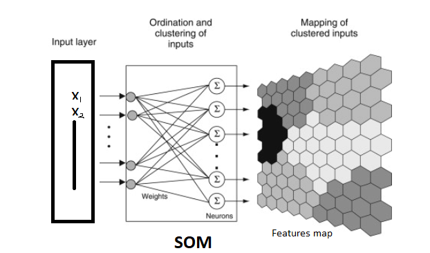
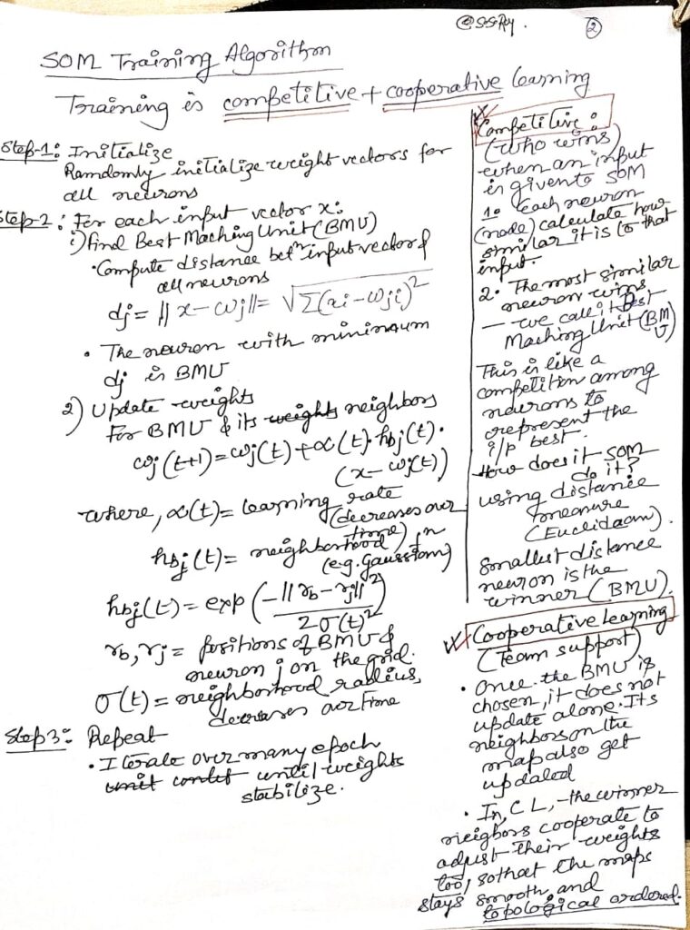
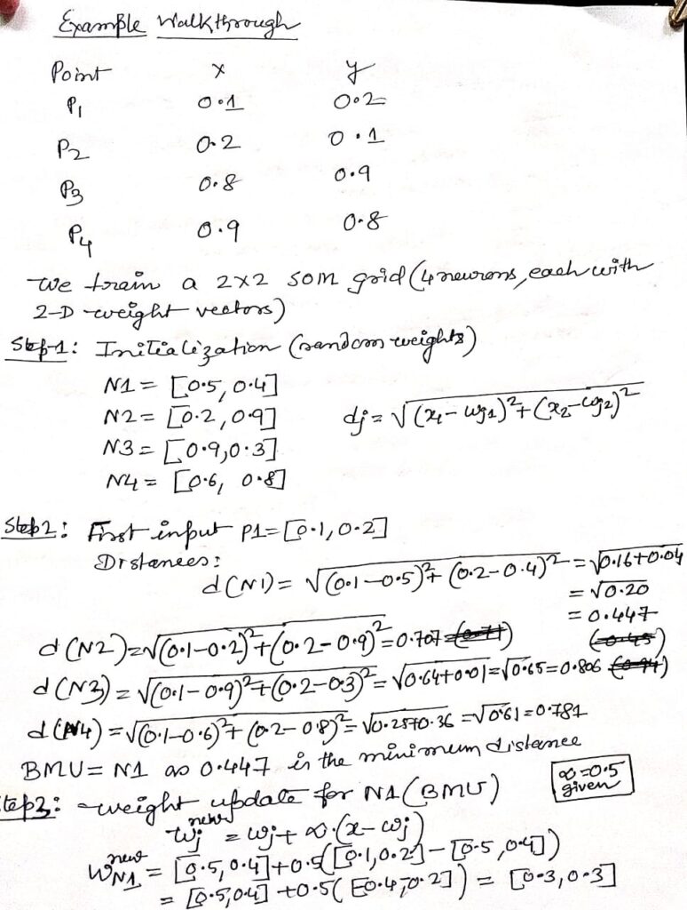
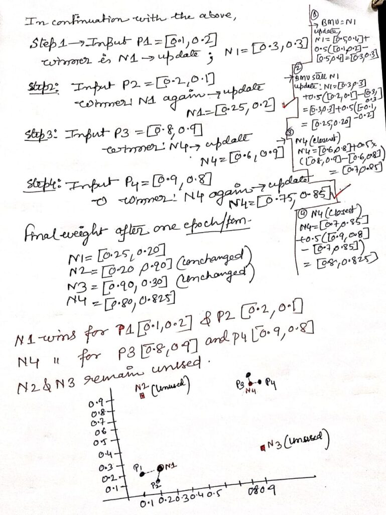
POINTS TO REMEMBER–>
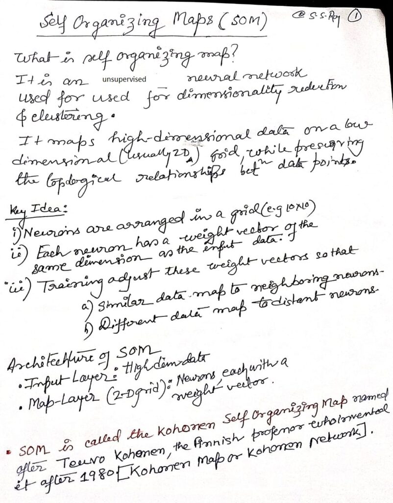
- Unsupervised neural network using competitive, neighborhood-based weight adaptation.
- Preserves topological relationships: nearby neurons map nearby inputs.
- Dimensionality reduction alternative to PCA, nonlinear manifold preserving.
- Converges via decreasing learning rate and shrinking neighborhood radius.
- Applications: clustering, visualization, anomaly detection, feature extraction.
- SOM scales poorly; parallel GPU/mini-batch training mitigates complexity.
- Topology choice (hexagonal vs rectangular grid) impacts neighborhood smoothing.
- Initialization (PCA-based vs random) strongly influences convergence stability.
- Quantization error and topographic error are key SOM evaluation metrics.
- Used for high-dimensional clustering in genomics, NLP embeddings, finance.
PCA
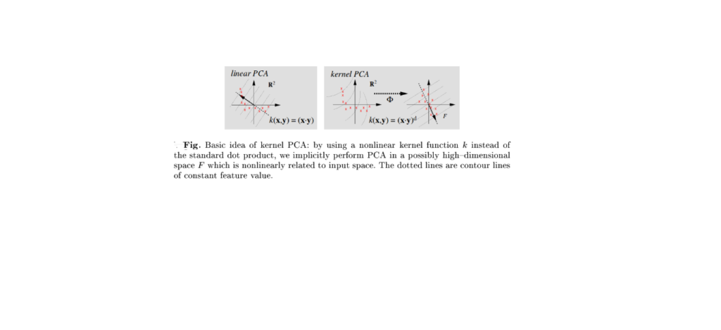
PCA (Principal Component Analysis) is a statistical method used to reduce the number of variables (dimensions) in a large dataset while retaining most of the original data’s variation and information. It does this by converting the data into new, independent variables called principal components, which help simplify complex data, improve visualizations, boost machine learning model performance, and make datasets easier to analyze and interpret.
PCA-KERNEL
t-SNE (t-distributed Stochastic Neighbor Embedding)
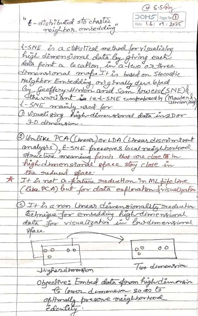
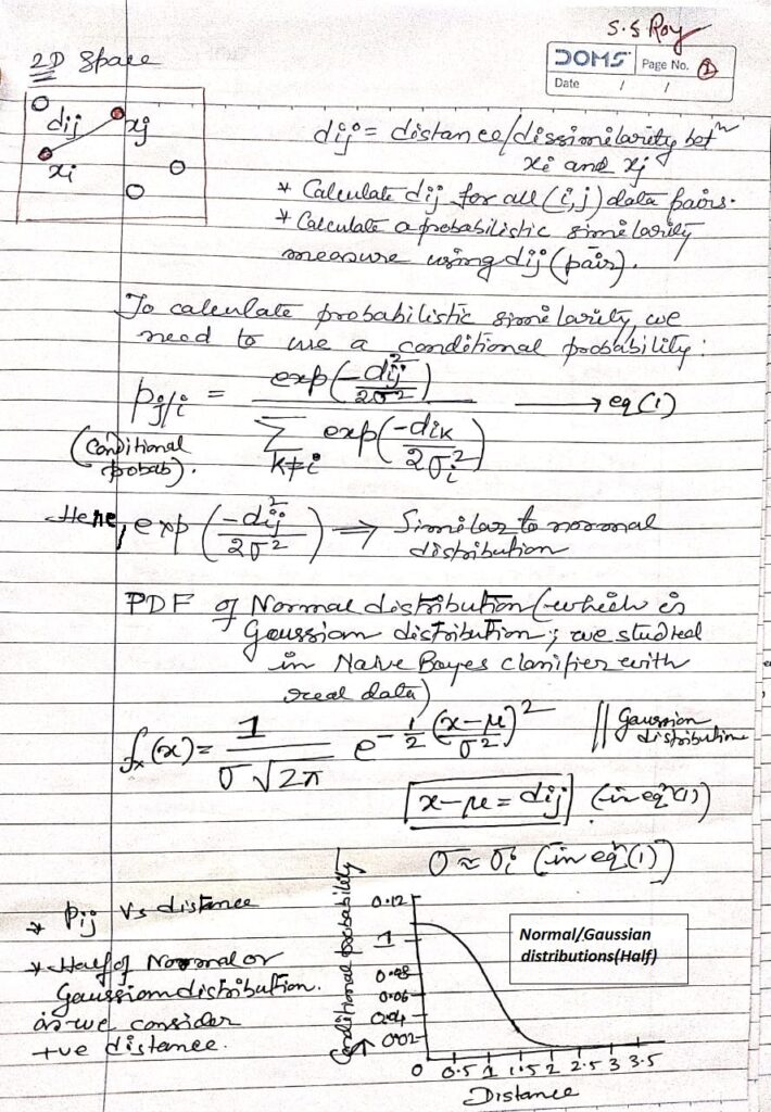
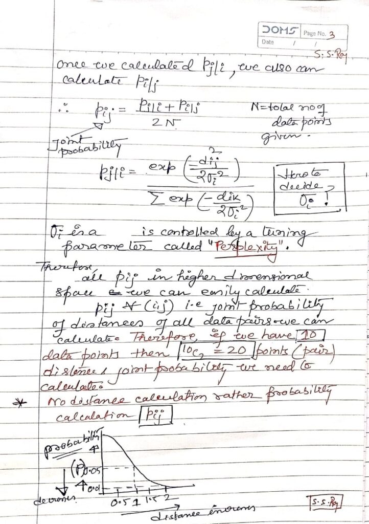
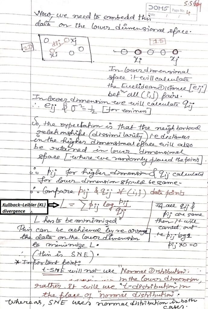
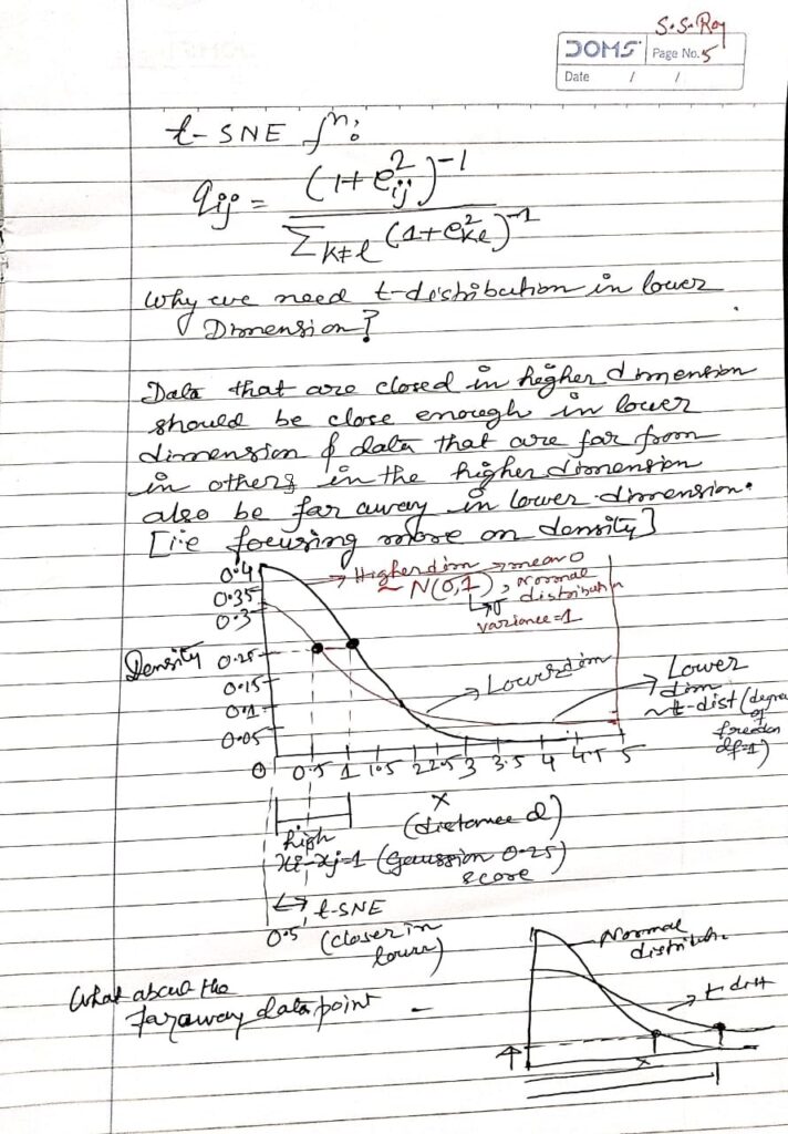
t-SNE (t-distributed Stochastic Neighbor Embedding), introduced by Laurens van der Maaten and Geoffrey Hinton (2008), is a non-linear dimensionality reduction technique, mainly used for visualizing high-dimensional data in 2D or 3D.
Important points->
How does perplexity influence structure?
→ Balances local detail vs. global cluster relationships.
Why Student-t distribution instead of Gaussian?
→ Heavy tails prevent crowding in low dimensions.
Why asymmetric KL-divergence?
→ Emphasizes preserving local neighborhoods more than global structure.
t-SNE vs. UMAP trade-offs?
→ UMAP faster, preserves global structure better than t-SNE.
Why not for downstream ML tasks?
→ Embeddings distort distances; unsuitable for predictive models.
Effect of initialization?
→ PCA gives stable maps; random can cause variability.
Scaling to millions of points?
→ Use Barnes-Hut or FFT approximations for efficiency.
Limitations of interpretability?
→ Global distances meaningless; only local clusters reliable.
Relation to manifold learning?
→ Captures local manifold structure via probabilistic similarities.
Misleading conclusions risk?
→ Wrong perplexity or iterations produce artificial clusters.
Kullback–Leibler (KL) divergence–>
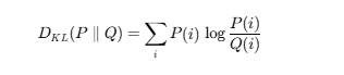
Kullback–Leibler (KL) divergence is an information-theoretic measure of how a probability distribution PPP diverges from a reference distribution Q. It is asymmetric, always non-negative, and equals zero only if P=Q. Widely used in t-SNE, variational inference, and generative models, KL-divergence quantifies information loss when approximating P with Q.
MATRIX DATA CALCULATION.*