Topics Covered
- Linked List : Singly,Doubly and Circular
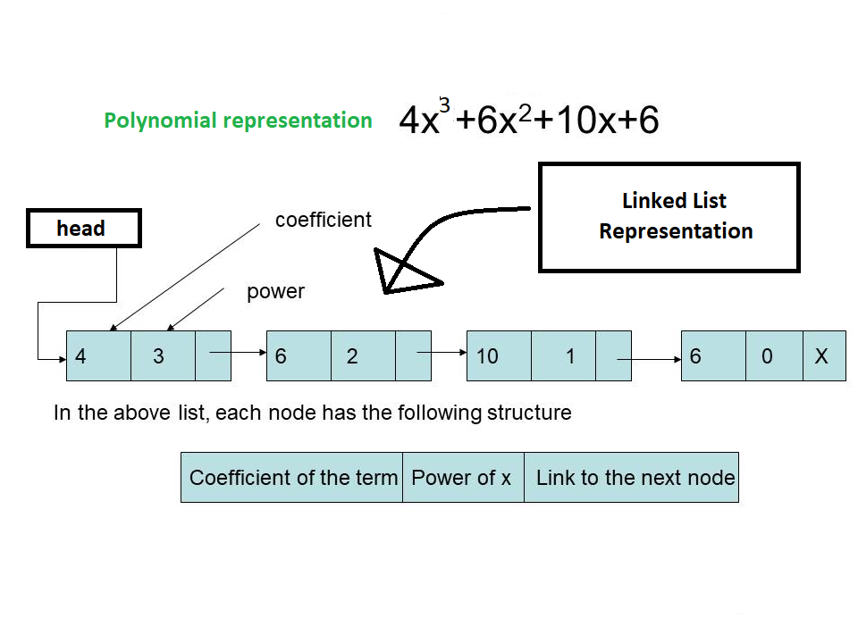
- Application of Linked List : Polynomial Representation and Addition
- Trees : Binary Tree, Binary Search Tree (finding kth smallest element)and Inorder, Pre-order and Post-Order Traversal in BST
- Special Tree: AVL Tree (Deletion)
- Hashing
Algorithms and data structures are the bedrock of computer science. They provide the methods and frameworks needed to process data efficiently, ensuring that software performs optimally under various conditions. An understanding of algorithms and data structures enables developers to create programs that are not only correct but also efficient and scalable.
Fundamentals of Algorithm Analysis
Algorithm analysis is a critical aspect of understanding and designing algorithms. It involves evaluating the performance of an algorithm, focusing primarily on its space and time complexity. These metrics help in determining how well an algorithm will perform as the input size increases and how it will utilize system resources.
Space Complexity
Space complexity refers to the amount of memory an algorithm needs to execute. It is an important factor in environments where memory is limited or where large data sets are involved. Space complexity is often divided into two parts:
- Fixed Part: This includes memory required by the algorithm that does not depend on the size of the input. For example, this could be the space needed for constants, static variables, and the program code itself.
- Variable Part: This includes memory that depends on the size of the input. For example, if an algorithm needs to create an array of size
nto store input data, the space complexity would increase linearly withn.
Example: a dynamic array to store n integers:
int* createArray(int n) {
    int* arr = (int*)malloc(n * sizeof(int));  // Dynamic array of size n
    return arr;
}- Space Complexity: The space complexity of this algorithm is O(n) because it requires memory proportional to the size of the input
n.
Another example is an algorithm that uses a fixed amount of memory regardless of the input size:
int sum(int a, int b) {
    return a + b;
}- Space Complexity: The space complexity here is O(1) (constant space) since the memory requirement does not change with the size of the input.
Time Complexity
Time complexity measures the amount of time an algorithm takes to complete as a function of the input size. It provides a way to estimate the running time of an algorithm, which is crucial for understanding how it will scale as the input size grows.
Time complexity is usually expressed using asymptotic notations, which provide a high-level understanding of the algorithm’s performance.
Types of Asymptotic Notations
- Big O Notation (O): Big O notation describes the upper bound of the time complexity. It represents the worst-case scenario, providing the maximum time an algorithm will take to complete as the input size increases.
- Example: For a simple linear search algorithm that searches for a value in an unsorted array of
nelements, the time complexity is O(n) because, in the worst case, the algorithm may have to check every element in the array.
   int linearSearch(int arr[], int n, int x) {
       for (int i = 0; i < n; i++) {
           if (arr[i] == x) {
               return i;
           }
       }
       return -1;
}- Omega Notation (Ω): Omega notation describes the lower bound of the time complexity. It represents the best-case scenario, giving the minimum time an algorithm will take to complete.
- Example: For the linear search algorithm above, the best-case time complexity is Ω(1), which occurs if the desired element is the first element in the array.
- Theta Notation (Θ): Theta notation provides a tight bound on the time complexity, meaning it gives both the upper and lower bounds. When the best-case and worst-case time complexities are the same, we use Theta notation.
Orders of Growth
The efficiency of an algorithm is also understood through its order of growth, which is how the time or space complexity of an algorithm increases as the input size increases.
- Constant Time – O(1): The algorithm’s performance is constant, and it does not depend on the input size.
- Example: Accessing a specific element in an array by index.
- Logarithmic Time – O(log n): The time complexity increases logarithmically with the input size.
- Example: Binary search algorithm, which divides the search space in half with each step.
- Linear Time – O(n): The time complexity increases linearly with the input size.
- Example: Linear search, where each element is checked one by one.
- Linearithmic Time – O(n log n): The time complexity increases in proportion to n log n. This is common in efficient sorting algorithms.
- Example: Merge sort or quicksort algorithms.
- Quadratic Time – O(n²): The time complexity increases quadratically with the input size.
- Example: A simple bubble sort algorithm, where each element is compared with every other element.
- Cubic Time – O(n³): The time complexity increases cubically with the input size.
- Example: Algorithms that involve three nested loops, such as matrix multiplication.
- Exponential Time – O(2^n): The time complexity doubles with each additional element in the input.
- Example: Algorithms that solve the traveling salesman problem through brute-force search.
- Factorial Time – O(n!): The time complexity increases factorially with the input size.
- Example: Algorithms that generate all possible permutations of a set.
Algorithm Efficiency: Best Case, Worst Case, Average Case
Understanding the best, worst, and average cases of an algorithm is essential for analyzing its performance in different scenarios.
- Best Case: This is the scenario where the algorithm performs the minimum number of operations. It is the most favorable outcome.
- Example: For a linear search, the best-case scenario occurs when the desired element is the first element in the array, giving a time complexity of O(1).
- Worst Case: This scenario represents the maximum number of operations the algorithm could perform. It is the least favorable outcome.
- Example: In the linear search algorithm, the worst-case occurs when the desired element is at the last position or not present at all, leading to a time complexity of O(n).
- Average Case: The average case represents the expected performance of the algorithm under typical conditions, assuming all inputs are equally likely. It provides a more realistic measure of the algorithm’s efficiency.
- Example: For linear search, assuming the desired element is equally likely to be at any position in the array, the average time complexity would be O(n/2), which simplifies to O(n).
Example: Binary Search Algorithm
To further illustrate these concepts, consider the binary search algorithm, which is used to find an element in a sorted array.
int binarySearch(int arr[], int n, int x) {
    int left = 0, right = n - 1;
    while (left <= right) {
        int mid = left + (right - left) / 2;
        if (arr[mid] == x) {
            return mid;  // Element found
        }
        if (arr[mid] < x) {
            left = mid + 1;
        } else {
            right = mid - 1;
        }
    }
    return -1;  // Element not found
}- Time Complexity:
- Best Case: O(1) – The element is found at the mid-point of the array in the first comparison.
- Worst Case: O(log n) – The algorithm reduces the search space by half with each iteration, so the maximum number of comparisons is logarithmic in relation to the array size.
- Average Case: O(log n) – On average, the element will be found after log n comparisons.
- Space Complexity: O(1) – The algorithm only requires a constant amount of additional memory, regardless of the input size.
Understanding the importance of algorithms and data structures, along with the concepts of space and time complexity, is crucial for developing efficient software. Through careful analysis using asymptotic notations and understanding different scenarios (best, worst, and average cases), developers can create algorithms that perform optimally, even as the size of the input grows. This knowledge is foundational for tackling more complex problems in computer science and engineering, leading to better, faster, and more scalable solutions.
Here’s a comparison of best case, worst case, and average case in a tabular format:
| Case | Description | Purpose | Example: Linear Search | Example: Binary Search |
|---|---|---|---|---|
| Best Case | The scenario where the algorithm performs the minimum number of operations. | Provides an optimistic view of the algorithm’s efficiency. | O(1): Desired element is the first in the array. | O(1): Desired element is at the middle. |
| Worst Case | The scenario where the algorithm performs the maximum number of operations. | Ensures the algorithm won’t exceed a particular performance threshold. | O(n): Desired element is the last or not present. | O(log n): Desired element is not in the array. |
| Average Case | The scenario representing the expected performance under typical conditions. | Offers a realistic estimate of the algorithm’s performance. | O(n): On average, the desired element could be anywhere in the array. | O(log n): Expected number of operations needed to find the element. |
This above table summarizes how each case reflects the algorithm’s performance in different situations, using linear search and binary search as examples.
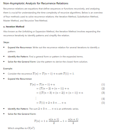
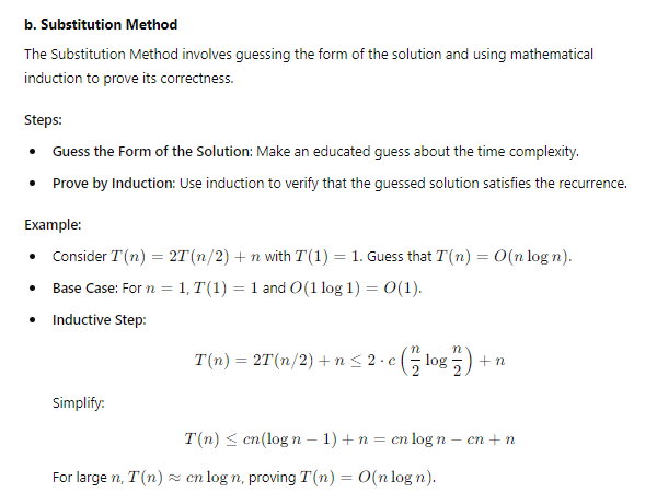
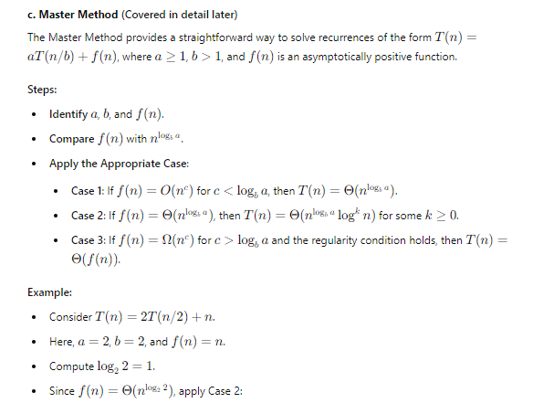
Recurrence Relation
Summary
- Iteration Method (a): Involves expanding the recurrence and identifying patterns.
- Substitution Method (b): Involves guessing the solution and proving it via induction.
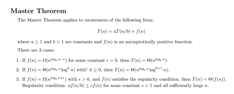
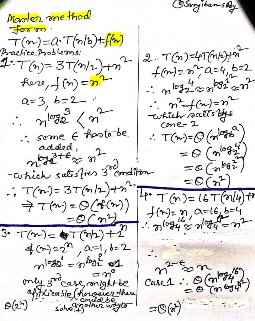
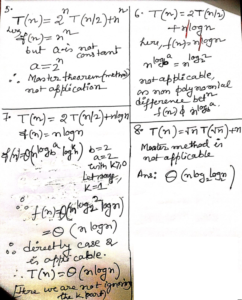
- Master Method (c): Provides a direct way to solve recurrences of the form ( T(n) = aT(n/b) + f(n) ).
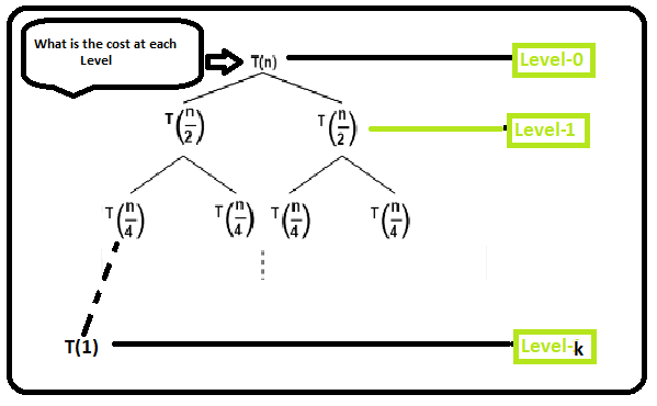
- Recursive Tree Method (d): Visualizes the recurrence as a tree to sum the costs at each level.
Each method has its own strengths and is suited to different types of recurrence relations. Understanding these methods provides a comprehensive toolkit for analyzing and solving recurrences in algorithmic problems.
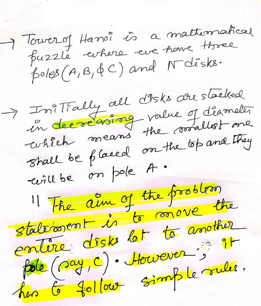
Application of Recursion : Tower of Hanoi
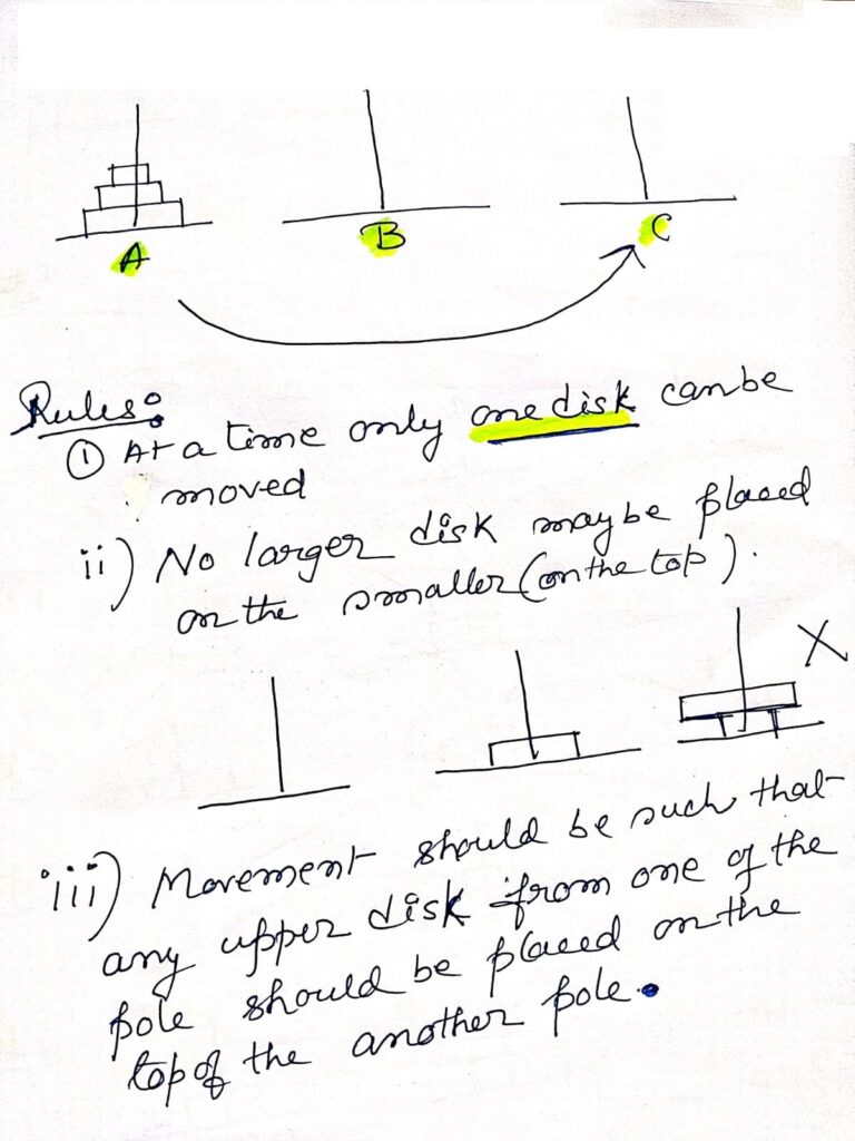
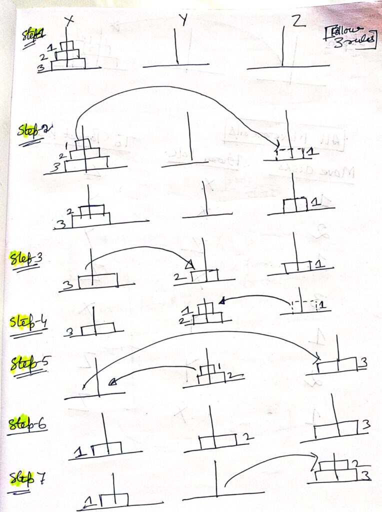
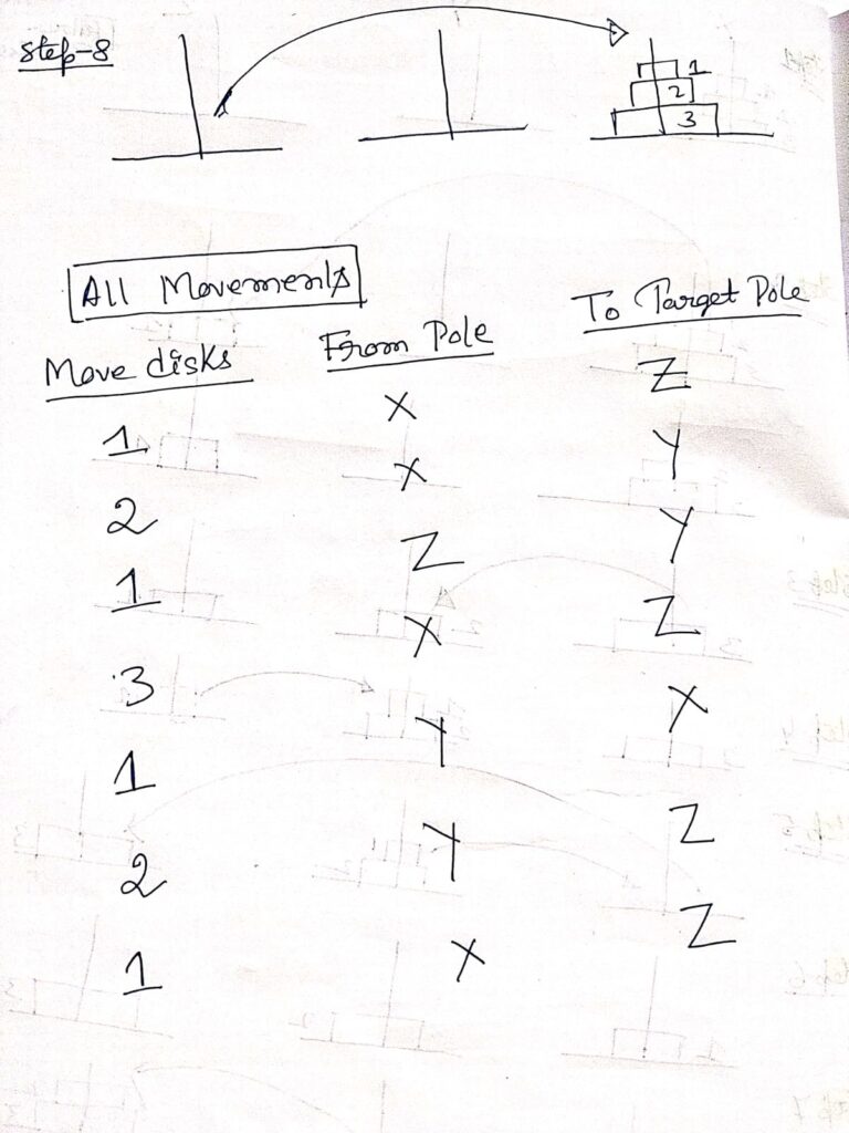
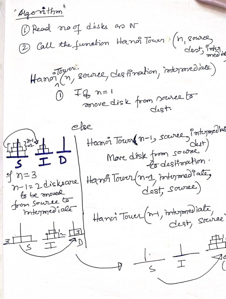
Time Complexity & Asymptotic Notations
Solving Recurrence Relation
Solving Recurrence Relation Using Master Method
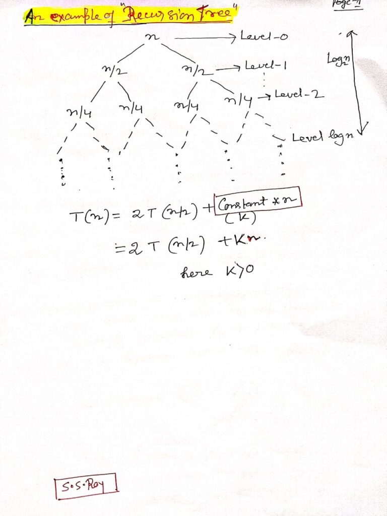
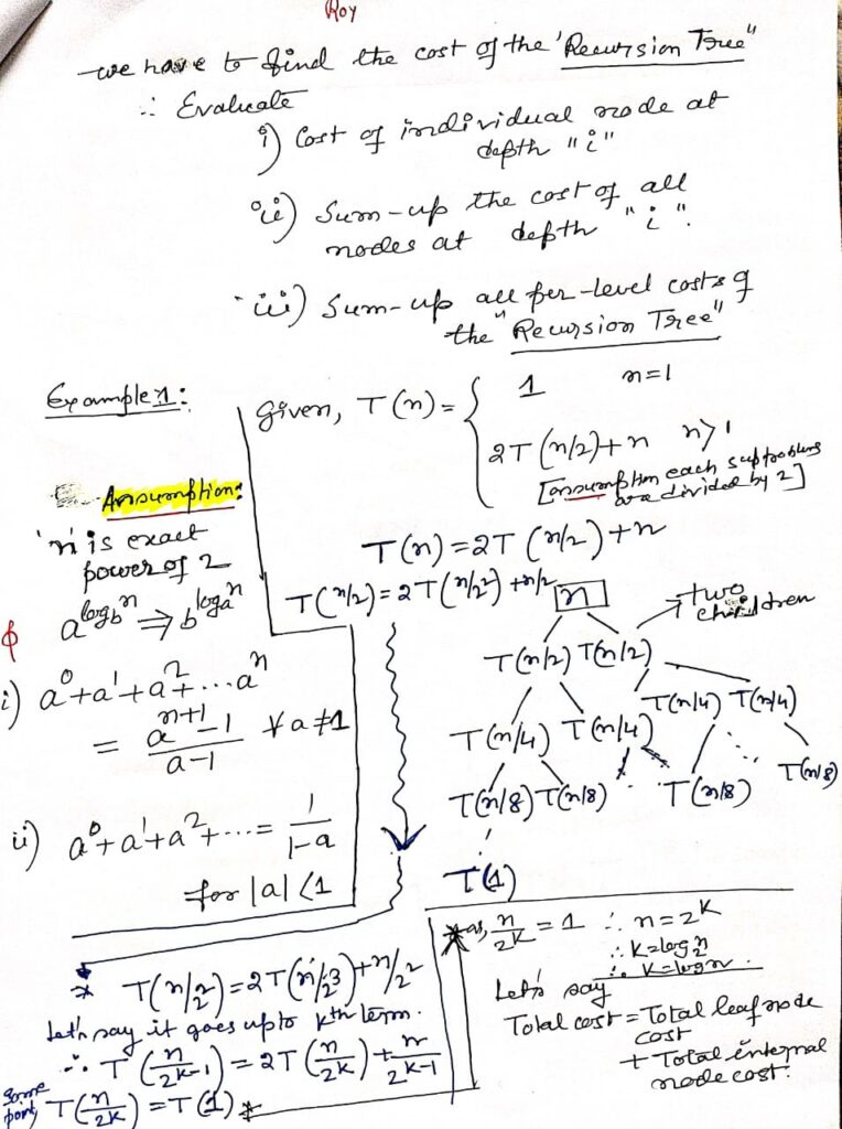
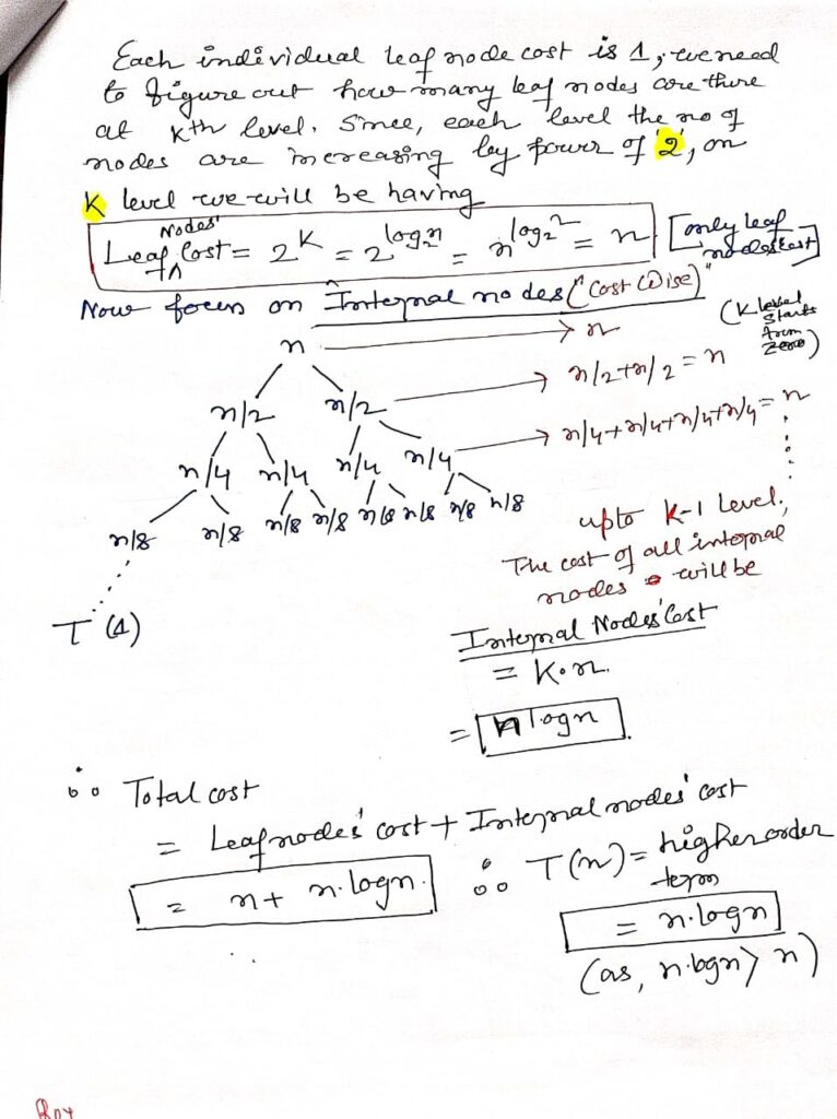
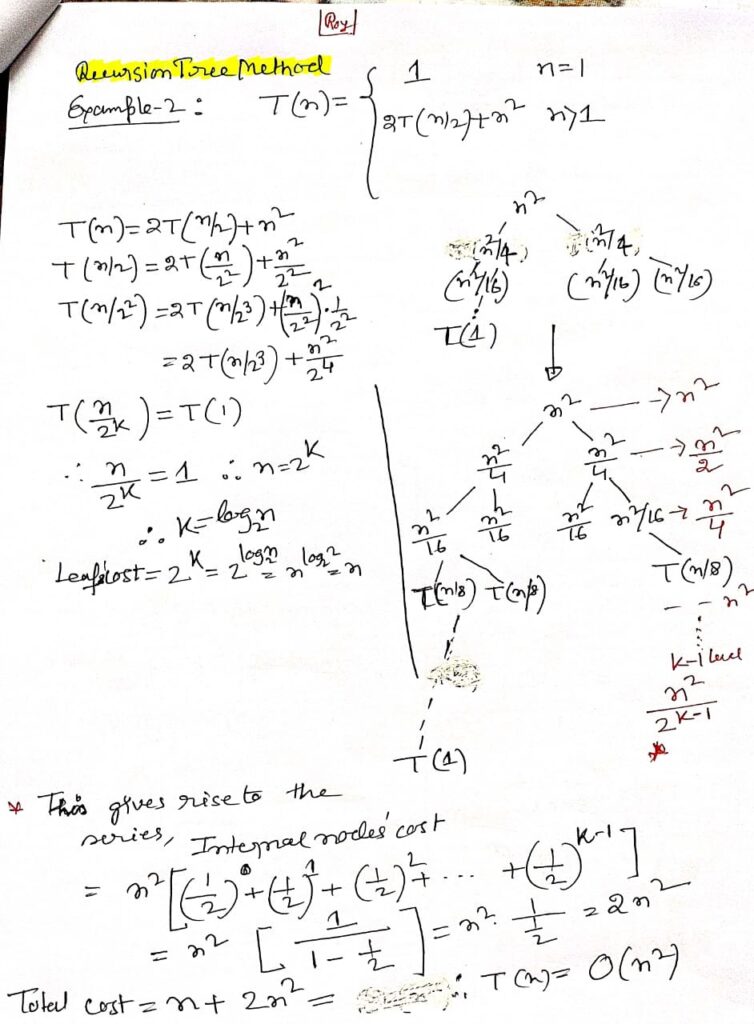
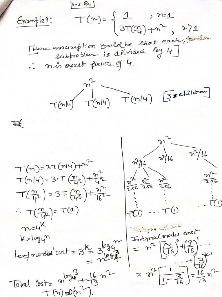
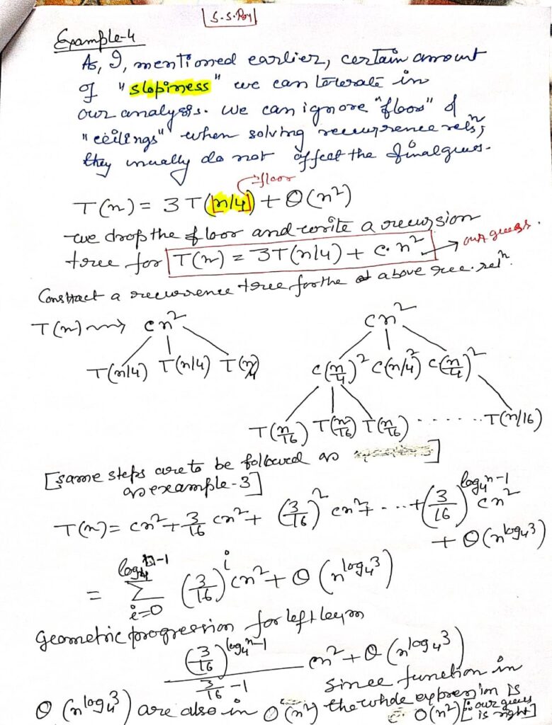
Solving Recurrence Relation Using Recursion Tree
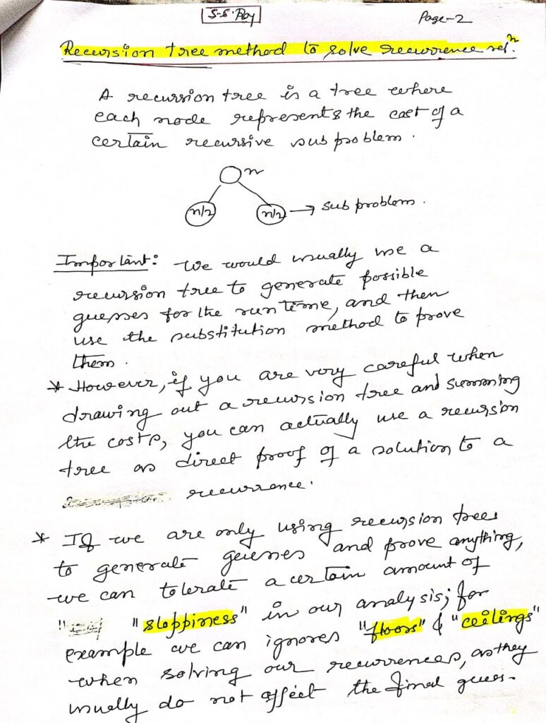
Recursion Tree Method
Recursion is a fundamental technique in computer science and mathematics that enables a function to call itself repeatedly, breaking down complex problems into more manageable sub-problems. One of the most effective ways to analyze and understand recursive algorithms is through a visual tool known as a recursion tree. This article will explore the concept of recursion trees, their structure, their role in time complexity analysis, and practical examples of how they are used to evaluate recursive functions.
What is a Recursion Tree?
A recursion tree is a diagrammatic representation that illustrates how a recursive function unfolds during its execution. It shows the different stages of recursive calls, how they branch out from one another, and how they eventually converge upon reaching the base case. By studying a recursion tree, one can gain a deeper understanding of the recursive process, its efficiency, and the computational resources it requires.
Structure of a Recursion Tree
In a recursion tree, each node represents a specific instance of a recursive call. The root node is the initial call to the function, while subsequent calls are represented as child nodes that branch out from the parent node. The number of branches emanating from a node is determined by the number of recursive calls made by the function at that stage. The depth of the tree reflects how many times the function recursively calls itself before reaching the base case.
Base Case:
The base case is the condition that halts the recursion. In a recursion tree, the nodes corresponding to the base case are typically leaf nodes, meaning they do not lead to further recursive calls. These nodes mark the point at which the recursive process begins to reverse, with the function returning values up the tree.
Recursive Calls:
Child nodes in the tree represent the recursive calls generated by the function. Each child node represents a smaller instance of the original problem, with different parameter values passed to the function. This recursive decomposition continues until all branches reach a base case.
To comprehend how a recursive function operates, it is useful to trace the execution flow through a recursion tree. Starting at the root node, you follow the branches to see how the function calls itself repeatedly, breaking the problem down into smaller parts. As the base cases are reached, the recursion begins to unwind, with each level of the tree returning values that contribute to the final solution.
Consider a recursive function that calculates the power of a number, for example:
def calculate_power(base, exponent):
    if exponent == 0:
        return 1
    return base * calculate_power(base, exponent - 1)
For an input of calculate_power(3, 4), the recursion tree would look like this:
    calculate_power(3, 4)
            |
    3 * calculate_power(3, 3)
            |
    3 * calculate_power(3, 2)
            |
    3 * calculate_power(3, 1)
            |
    3 * calculate_power(3, 0)
            |
            1
This recursion tree demonstrates that each recursive call reduces the exponent by one until the base case exponent == 0 is reached, at which point the recursion halts, and the values are returned up the tree.
Time Complexity Analysis Using Recursion Trees
Recursion trees are invaluable for analyzing the time complexity of recursive algorithms. By examining the tree’s structure, we can determine the number of recursive calls made at each level and the amount of work done at each step. This analysis is crucial for understanding the overall efficiency of an algorithm and identifying areas for potential optimization.
Linear Recursion Example:
Consider a function that calculates the sum of integers from 1 to n. The pseudo-code might look like this:
def sum_integers(n):
    if n == 0:
        return 0
    return n + sum_integers(n - 1)
The recursion tree for sum_integers(4) would appear as follows:
    sum_integers(4)
            |
    4 + sum_integers(3)
            |
    3 + sum_integers(2)
            |
    2 + sum_integers(1)
            |
    1 + sum_integers(0)
            |
            0
This is an example of linear recursion, where each function call leads to exactly one subsequent call. The time complexity is O(n), as the function makes n recursive calls.
Tree Recursion Example:
Tree recursion occurs when a function makes multiple recursive calls within each execution. A classic example is the calculation of Fibonacci numbers. Here’s a simplified version:
def fibonacci(n):
    if n <= 1:
        return n
    return fibonacci(n - 1) + fibonacci(n - 2)
The recursion tree for fibonacci(4) would look like this:
            fibonacci(4)
               /    \
       fibonacci(3)  fibonacci(2)
          /   \        /   \
  fibonacci(2) fibonacci(1) fibonacci(1) fibonacci(0)
     /   \
fibonacci(1) fibonacci(0)
In this example, each recursive call generates two further calls, leading to an exponential growth in the number of calls. The time complexity for this tree recursion is O(2^n), which makes it less efficient for large inputs.
The Recursion Tree Method in Depth
The recursion tree method is a powerful technique for solving recurrence relations that define the time complexity of recursive algorithms. Recurrence relations are mathematical expressions that describe the overall time required by a recursive algorithm in terms of the time required by smaller sub-problems.
Example:
Consider the recurrence relation T(n) = 2T(n/2) + O(n), which might describe the time complexity of the Merge Sort algorithm. The recursion tree for this relation would help us understand that each level of the tree performs O(n) work, and the total height of the tree is log n, leading to an overall time complexity of O(n log n).
The binary search algorithm, on the other hand, is described by the recurrence relation T(n) = T(n/2) + O(1). The recursion tree for this relation shows that each level of the tree reduces the problem size by half, resulting in a logarithmic time complexity O(log n).
Practical Applications of Recursion Trees
Recursion trees are not just theoretical constructs; they have practical applications in analyzing and optimizing algorithms in various domains, including sorting, searching, and dynamic programming.
Sorting Algorithms:
In sorting algorithms like Quick Sort and Merge Sort, recursion trees help visualize how the array is repeatedly divided into smaller sub-arrays and then merged or sorted. This visualization aids in understanding the time complexity and guiding optimization efforts.
Dynamic Programming:
In dynamic programming, recursion trees help identify overlapping sub-problems, which can then be optimized using memoization or tabulation. This prevents the exponential growth of recursive calls and reduces the time complexity from exponential to polynomial.
Divide and Conquer:
Recursion trees are integral to analyzing divide-and-conquer algorithms, where a problem is divided into smaller sub-problems, each solved recursively. Understanding the recursion tree helps determine how efficiently the problem is being divided and combined.
The recursion tree method is a valuable tool for understanding and analyzing recursive algorithms. By breaking down the execution of a recursive function into a tree structure, we can visualize its behavior, assess its time complexity, and optimize its performance. Whether dealing with simple linear recursion or more complex tree recursion, mastering the recursion tree method is essential for computer scientists, mathematicians, and anyone working with algorithms.
Stacks and Queues
Stack Data Structure: Detailed Overview

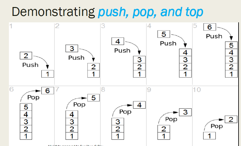
A stack is a fundamental data structure used extensively in computer science and programming. It operates on a Last In, First Out (LIFO) principle, meaning that the most recently added element is the first one to be removed. This characteristic makes stacks particularly useful in scenarios where the most recent data needs to be accessed first.
Stacks
1. Basic Operations:
- Push: This operation adds an element to the top of the stack. It is often implemented by incrementing the top index or adding a new node in the linked list-based implementation.
- Pop: This operation removes the element from the top of the stack. It updates the top index or the head pointer of the linked list and returns the removed element.
- Peek (or Top): This operation retrieves the element at the top of the stack without removing it. It allows access to the most recent element without altering the stack.
- IsEmpty: This function checks if the stack is empty. It returns true if there are no elements in the stack and false otherwise.
2. Implementation:
Stacks can be implemented using arrays or linked lists. Each implementation has its own advantages and constraints.
- Array-based Implementation: In this approach, a fixed-size array is used to represent the stack. The key component is an integer index, often called
top, which keeps track of the index of the top element. Thepushoperation increments this index and places the new element at that position, while thepopoperation decrements the index. This method has a fixed capacity, making it essential to manage the stack size carefully to avoid overflow.
3. Applications:
- Expression Evaluation: Stacks are used to evaluate expressions, particularly in postfix (Reverse Polish Notation) and infix notations. For instance, converting infix expressions to postfix or evaluating postfix expressions involves using stacks to manage operators and operands.
- Backtracking: Algorithms that require backtracking, such as depth-first search (DFS), use stacks to remember the path taken. Stacks help revert to the previous state by popping elements off the stack, enabling the exploration of alternative paths.
- Function Call Management: The call stack manages function calls and local variables in programming languages. It tracks the order of function calls and supports recursion by storing return addresses and local variables for each call.
4. Performance Considerations:
- Time Complexity: Stack operations, including push, pop, and peek, operate in O(1) time. This constant time complexity is due to the direct access and modification of the top element.
- Space Complexity: The space complexity is O(n), where
nis the number of elements in the stack. Both array-based and linked list-based implementations require space proportional to the number of elements stored.
5. Common Pitfalls:
- Overflow and Underflow:
- Overflow: In array-based stacks, pushing an element onto a full stack results in overflow. Proper checks and resizing strategies are required to manage capacity.
- Underflow: Popping an element from an empty stack leads to underflow. Implementing checks to ensure the stack is not empty before popping is crucial.
6. Practical Examples:
- Undo Mechanism in Applications: Many software applications implement undo functionality using stacks. Each action is pushed onto the stack, and undoing an action involves popping the most recent action and reversing it.
- Balanced Parentheses Checking: Stacks are used to check for balanced parentheses in expressions or code snippets. Each opening parenthesis is pushed onto the stack, and each closing parenthesis triggers a pop operation, ensuring all parentheses are correctly matched.
By understanding and utilizing stacks effectively, you can solve a variety of computational problems efficiently. Stacks provide a robust method for managing data with a LIFO ordering, making them an essential component of many algorithms and systems.
A sample C code for Stack:
#include <stdio.h>
#define MAX 100 // Define the maximum size of the stack

// Structure to represent a stack
typedef struct {
    int top; // Index of the top element
    int arr[MAX]; // Array to hold stack elements
} Stack;

// Function to initialize the stack
void initialize(Stack *s) {
    s->top = -1; // Set top to -1 indicating the stack is empty
}

// Function to check if the stack is empty
int isEmpty(Stack *s) {
    return s->top == -1;
}

// Function to check if the stack is full
int isFull(Stack *s) {
    return s->top == MAX - 1; // Use - instead of an incorrect dash symbol
}

// Function to add an element to the stack
void push(Stack *s, int value) {
    if (isFull(s)) {
        printf("Stack overflow. Cannot push %d\n", value);
        return;
    }
    s->arr[++(s->top)] = value; // Increment top and add the element
    printf("%d pushed to stack\n", value);
}

// Function to remove an element from the stack
int pop(Stack *s) {
    if (isEmpty(s)) {
        printf("Stack underflow. Cannot pop\n");
        return -1; // Return a sentinel value to indicate failure
    }
    return s->arr[(s->top)--]; // Return the top element and decrement top
}

// Function to get the top element of the stack without removing it
int peek(Stack *s) {
    if (isEmpty(s)) {
        printf("Stack is empty\n");
        return -1; // Return a sentinel value to indicate failure
    }
    return s->arr[s->top]; // Return the top element
}

// Function to display the elements of the stack
void display(Stack *s) {
    if (isEmpty(s)) {
        printf("Stack is empty\n");
        return;
    }
    printf("Stack elements are:\n");
    for (int i = s->top; i >= 0; i--) { // Use -- instead of an incorrect dash symbol
        printf("%d\n", s->arr[i]);
    }
}

// Main function to demonstrate stack operations
int main() {
    Stack s;
    initialize(&s); // Initialize the stack

    // Demonstrate stack operations
    push(&s, 10);
    push(&s, 20);
    push(&s, 30);
    display(&s);

    printf("%d popped from stack\n", pop(&s));
    display(&s);

    printf("Top element is %d\n", peek(&s));

    return 0;
}
Queue and Circular Queue: Detailed Explanation
1. Linear Queue
Definition:
A queue is a linear data structure that follows the First In, First Out (FIFO) principle. This means that the first element added to the queue will be the first one to be removed.
Operations:
- Enqueue: Adds an element to the rear of the queue.
- Dequeue: Removes an element from the front of the queue.
- Front (Peek): Retrieves the element at the front of the queue without removing it.
- IsEmpty: Checks whether the queue is empty.
- IsFull: Checks whether the queue is full (for array-based implementation).
Applications:
- Task Scheduling: Manages tasks in the order they arrive, such as print jobs or CPU task scheduling.
- Data Buffers: Manages data streams where the order of processing is crucial.
- Breadth-First Search (BFS): Used in BFS algorithms to explore nodes level by level.
Array-Based Implementation:
Diagram:
Queue:
Front -> | 1 | <- Front (first element to be removed)
         | 2 |
         | 3 |
         | 4 | <- Rear (most recent element added)
Code Example:
#include <stdio.h>
#include <stdlib.h>

#define MAX 100 // Maximum size of the queue

typedef struct {
    int front, rear, size;
    int arr[MAX];
} Queue;

// Initialize the queue
void initialize(Queue *q) {
    q->front = 0;
    q->rear = -1;
    q->size = 0;
}

// Check if the queue is empty
int isEmpty(Queue *q) {
    return q->size == 0;
}

// Check if the queue is full
int isFull(Queue *q) {
    return q->size == MAX;
}

// Add an element to the queue
void enqueue(Queue *q, int value) {
    if (isFull(q)) {
        printf("Queue is full. Cannot enqueue %d\n", value);
        return;
    }
    q->rear =
2.Circular Queue
**Definition:**
A circular queue is a variation of the standard queue where the end of the queue wraps around to the beginning, effectively making the queue circular. This implementation overcomes the limitations of a linear array-based queue where elements may leave gaps.
**Operations:**
– Enqueue: Adds an element to the rear of the queue.
– Dequeue: Removes an element from the front of the queue.
– Front (Peek): Retrieves the element at the front without removing it.
– IsEmpty: Checks if the queue is empty.
– IsFull: Checks if the queue is full.
Circular Queue (Max Size: 5):
Front -> | 1 | <- Front (first element to be removed)
| 2 |
| 3 |
| 4 |
| 5 | <- Rear (most recent element added)
After enqueue operations, the queue wraps around:
Front -> | 6 |
| 7 |
| 8 |
| 9 |
| 10| <- Rear
Circular Queue
Here is a complete C code implementation for a circular queue. This implementation uses an array to store the elements and maintains the front, rear, and size to manage the queue operations.
#include <stdio.h>
#include <stdlib.h>

#define MAX 5 // Define the maximum size of the circular queue

typedef struct {
    int front, rear, size;
    int arr[MAX];
} CircularQueue;

// Initialize the circular queue
void initialize(CircularQueue *q) {
    q->front = 0;
    q->rear = -1;
    q->size = 0;
}

// Check if the circular queue is empty
int isEmpty(CircularQueue *q) {
    return q->size == 0;
}

// Check if the circular queue is full
int isFull(CircularQueue *q) {
    return q->size == MAX;
}

// Add an element to the circular queue
void enqueue(CircularQueue *q, int value) {
    if (isFull(q)) {
        printf("Queue is full. Cannot enqueue %d\n", value);
        return;
    }
    q->rear = (q->rear + 1) % MAX; // Update rear index circularly
    q->arr[q->rear] = value;
    q->size++;
    printf("%d enqueued to queue\n", value);
}

// Remove an element from the circular queue
int dequeue(CircularQueue *q) {
    if (isEmpty(q)) {
        printf("Queue is empty. Cannot dequeue\n");
        return -1; // Sentinel value indicating error
    }
    int value = q->arr[q->front];
    q->front = (q->front + 1) % MAX; // Update front index circularly
    q->size--;
    return value;
}

// Retrieve the front element without removing it
int front(CircularQueue *q) {
    if (isEmpty(q)) {
        printf("Queue is empty\n");
        return -1; // Sentinel value indicating error
    }
    return q->arr[q->front];
}

// Display the elements of the circular queue
void display(CircularQueue *q) {
    if (isEmpty(q)) {
        printf("Queue is empty\n");
        return;
    }
    printf("Queue elements are:\n");
    for (int i = 0; i < q->size; i++) {
        printf("%d\n", q->arr[(q->front + i) % MAX]);
    }
}

// Main function to demonstrate circular queue operations
int main() {
    CircularQueue q;
    initialize(&q);

    enqueue(&q, 10);
    enqueue(&q, 20);
    enqueue(&q, 30);
    enqueue(&q, 40);
    enqueue(&q, 50);
    display(&q);

    printf("%d dequeued from queue\n", dequeue(&q));
    printf("%d dequeued from queue\n", dequeue(&q));
    display(&q);

    enqueue(&q, 60);
    enqueue(&q, 70);
    display(&q);

    printf("Front element is %d\n", front(&q));

    return 0;
}
Explanation:
- Structure Definition:
CircularQueuestructure contains:front: Index of the first element.rear: Index of the last element.size: Number of elements in the queue.arr[MAX]: Array to store the elements.
- Initialization:
initialize()setsfrontto 0,rearto -1, andsizeto 0.
- Check Functions:
isEmpty()returns true if the queue has no elements.isFull()returns true if the queue is full.
- Enqueue Operation:
enqueue()adds an element to the rear of the queue. Therearindex is updated circularly using modulo arithmetic.
- Dequeue Operation:
dequeue()removes an element from the front of the queue. Thefrontindex is updated circularly using modulo arithmetic.
- Front Operation:
front()retrieves the front element without removing it.
- Display Function:
display()prints all elements from the front to the rear in the circular queue.
- Main Function:
- Demonstrates operations by enqueuing and dequeuing elements, and displaying the queue’s contents.
This implementation ensures that the circular queue efficiently manages the elements, utilizing the available space effectively.
Summary of Stack data structure.
Origin
- Introduced by Alan M. Turing in 1946 using the terms “bury” and “unbury” for subroutines
- Formally proposed by Klaus Samelson and Friedrich L. Bauer in 1955; patent filed in 1957
- Bauer received the IEEE Computer Pioneer Award in 1988 for the stack principle
Key Characteristics
- LIFO (Last-In-First-Out) data structure
- Push: Adding an item to the stack
- Pop: Removing an item from the stack
- Access is only at the top
Applications
- Conversion of Infix to Postfix or Prefix expressions
- Backtracking techniques
- Function call and return processes
- Saving local variables during nested function calls
- Web browser page-visited history
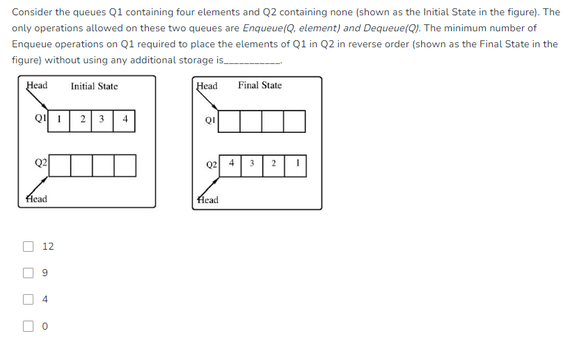
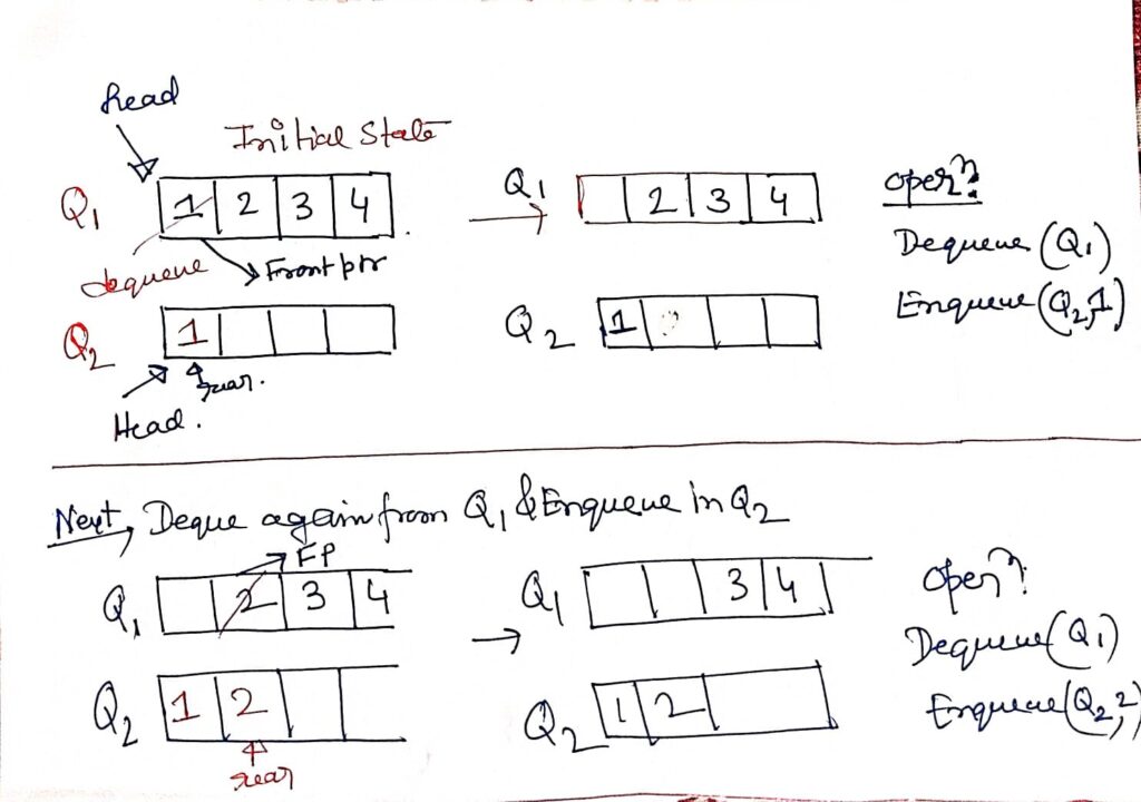
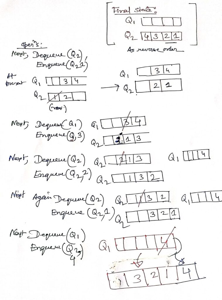
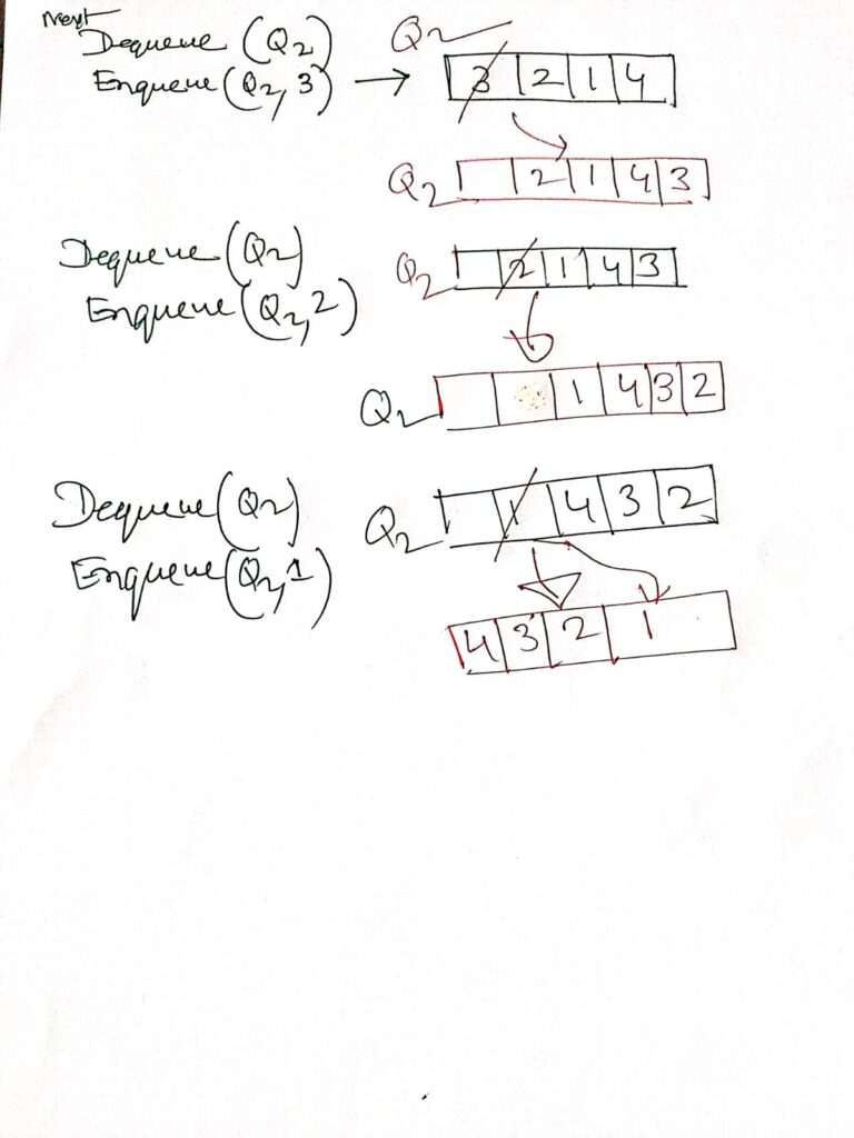
Summary of QUEUE and Circular Queue
Understanding Expression Notations: Infix, Prefix, and Postfix
What are Expression Notations?
Expression notations are different ways to represent mathematical operations. These notations determine the placement of operators relative to their operands.
Infix Notation
In infix notation, the operator is positioned between its operands. This is the most commonly used format in everyday arithmetic.
- Example: 2 + 3
Postfix Notation
Postfix notation, also known as Reverse Polish Notation (RPN), places the operator after its operands.
- Example: 2 3 +
Prefix Notation
Prefix notation, or Polish Notation, positions the operator before its operands.
- Example: + 2 3
Evaluating Expressions
The method for evaluating each notation differs.
- Infix: Requires considering operator precedence and parentheses to determine the order of operations.
- Postfix: Typically involves using a stack data structure to process the expression from left to right.
- Prefix: Similar to postfix, but evaluation proceeds from right to left using a stack.
Advantages and Disadvantages
- Infix: Easy to read for humans but can be complex for computers to process.
- Postfix and Prefix: Often more efficient for computer processing as they eliminate the need for parentheses and complex precedence rules. However, they can be less intuitive for humans to understand.
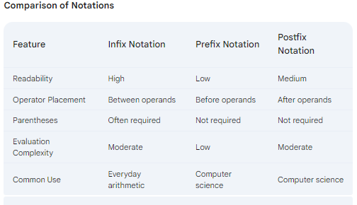
Conversion and Efficiency
It’s possible to convert between different notations. For example, infix expressions can be transformed into postfix or prefix form using algorithms like the Shunting Yard algorithm. Postfix and prefix notations generally offer performance advantages in computer applications due to their simpler evaluation process.
Choosing the Right Notation
The optimal notation depends on the specific application. Infix is preferred for human interaction, while postfix and prefix are often used in programming and compiler design for efficient expression handling.
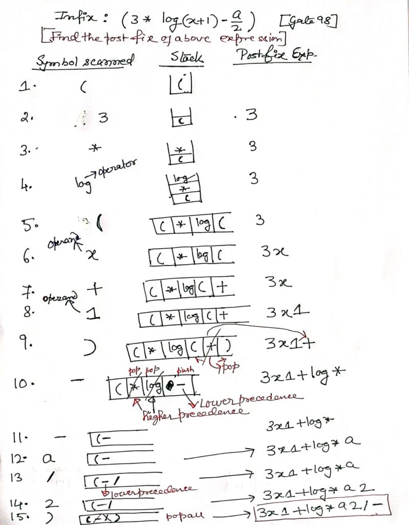
Infix to Postfix Conversion
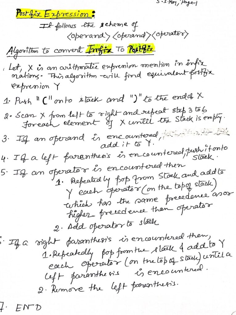
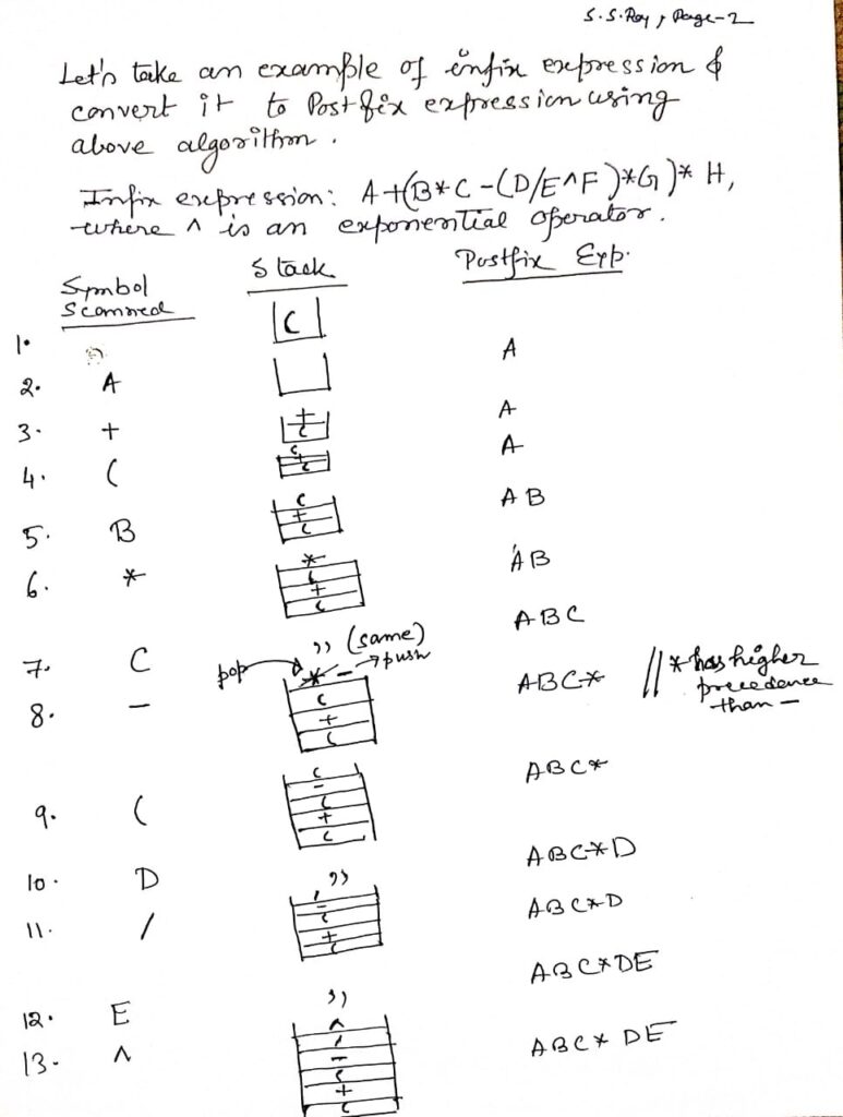
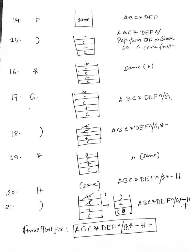
Infix to prefix conversion
To transform an infix expression into a prefix expression, you can follow these steps using a stack data structure:
- Reverse the Infix Expression: Start by reversing the original infix expression. As you reverse, swap every opening parenthesis
(with a closing parenthesis)and vice versa. - Convert the Reversed Infix to a “Near-Postfix” Expression: Next, process the reversed infix expression to obtain a postfix expression. However, when you handle operators during this conversion, only pop operators from the stack if they have strictly greater precedence than the current operator (rather than popping for equal or greater precedence).
- Reverse the Resulting Expression: Finally, take the postfix expression generated in the previous step and reverse it to obtain the desired prefix expression.
Throughout the process, the stack is utilized to facilitate the conversion from infix to postfix, which is then adjusted to generate the prefix form.
Let’s go through the process of converting the infix expression (A + B) * (C - D) to prefix notation, showing the stack at each step.
Step 1: Reverse the Infix Expression
- Original infix:
(A + B) * (C - D) - Reversed expression:
(D - C) * (B + A)
Step 2: Replace Each Parenthesis
- Replace
(with)and vice versa in the reversed expression. - After replacement:
)D - C( * )B + A(
Step 3: Convert the Modified Expression to Postfix
Now we’ll convert )D - C( * )B + A( to postfix notation, showing the stack at each step.
- Scan
):
- Stack:
) - Postfix Expression:
- Scan
D:
- Stack:
) - Postfix Expression:
D
- Scan
-:
- Stack:
) - - Postfix Expression:
D
- Scan
C:
- Stack:
) - - Postfix Expression:
DC
- Scan
((pop until)):
- Pop
-and add to postfix. - Stack:
- Postfix Expression:
DC-
- Scan
*:
- Stack:
* - Postfix Expression:
DC-
- Scan
):
- Stack:
* ) - Postfix Expression:
DC-
- Scan
B:
- Stack:
* ) - Postfix Expression:
DC-B
- Scan
+:
- Stack:
* ) + - Postfix Expression:
DC-B
- Scan
A:- Stack:
* ) + - Postfix Expression:
DC-BA
- Stack:
- Scan
((pop until)):- Pop
+and add to postfix. - Stack:
* - Postfix Expression:
DC-BA+
- Pop
- Pop remaining operators:
- Pop
*and add to postfix. - Stack:
- Postfix Expression:
DC-BA+*
- Pop
Step 4: Reverse the Postfix Expression
- Reverse the postfix expression
DC-BA+*to obtain the prefix expression. - Reversed postfix:
*+AB-CD
Final Prefix Expression
The final prefix expression for the given infix expression (A + B) * (C - D) is *+AB-CD.
Search Techniques
Search algorithms are fundamental in computer science for locating specific data within a collection. There are various search algorithms, each with different efficiencies depending on the data structure and size. Two common search methods are linear search and binary search.
- Linear Search:
- Description: Linear search is the simplest search algorithm. It checks each element in the array until the target value is found or the array ends. It’s effective for small or unsorted datasets.
- Time Complexity: O(n), where n is the number of elements in the array.
- Binary Search:
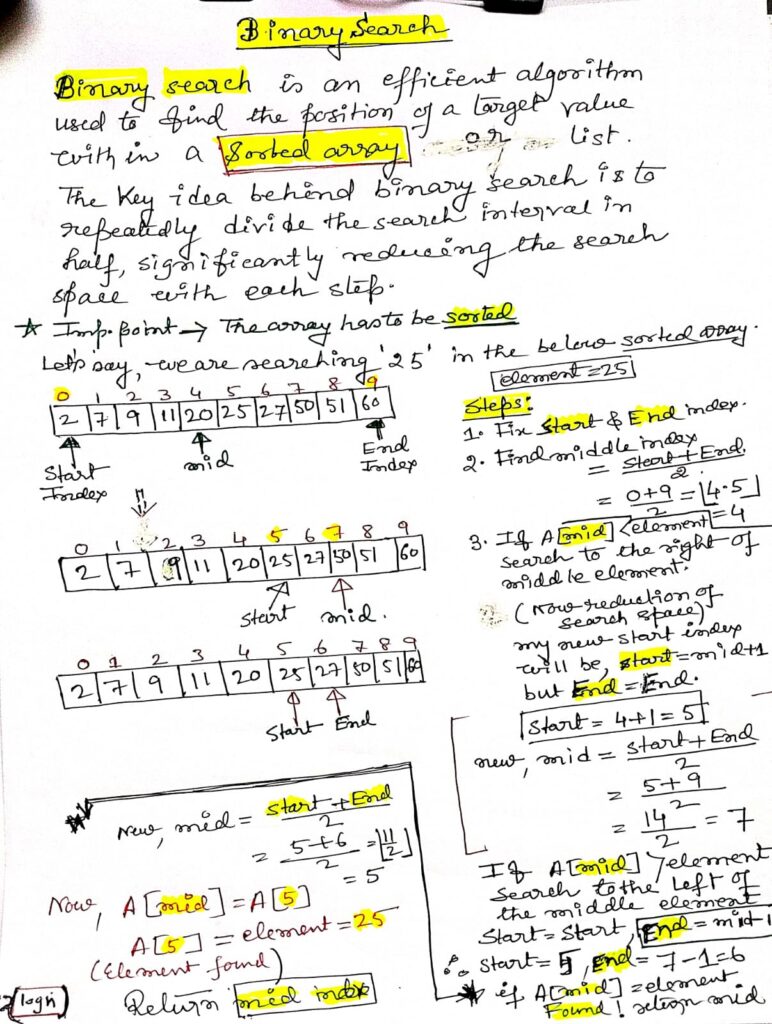
- Description: Binary search is more efficient but requires the array to be sorted. It works by repeatedly dividing the search interval in half. If the target value is less than the middle element, the search continues in the left half, otherwise in the right half.
- Time Complexity: O(log n), making it significantly faster for large, sorted datasets.
Here’s a simple C program implementing the linear search algorithm:
#include <stdio.h>

// Function to perform linear search
int linearSearch(int arr[], int n, int target) {
    for (int i = 0; i < n; i++) {
        if (arr[i] == target) {
            return i; // Return the index of the target element
        }
    }
    return -1; // Return -1 if the element is not found
}

int main() {
    int arr[] = {10, 25, 30, 45, 60, 75};
    int n = sizeof(arr) / sizeof(arr[0]);
    int target = 45;

    int result = linearSearch(arr, n, target);

    if (result != -1) {
        printf("Element found at index %d\n", result);
    } else {
        printf("Element not found in the array\n");
    }

    return 0;
}
Explanation:
linearSearchFunction: Iterates through each element of the array to find the target value. If the target is found, the function returns the index; otherwise, it returns-1.mainFunction: Initializes an array and the target value to search for. It then callslinearSearchand prints the result.
Output:
If the target value 45 is in the array, the program will output:
Element found at index 3If the target value is not in the array, it will output:
Element not found in the array
Linked List
Applications of Linked List : Polynomial Representation & Addition
Linear Search
Linear Search:
Linear Search is a straightforward search algorithm that traverses each element of a list or array sequentially to locate a target value. It works by comparing the target with each element in the array one by one until the target is found or all elements are checked.
Key Characteristics:
- Unsorted Data: It can search in both sorted and unsorted data.
- Simplicity: Easy to implement and understand.
- Time Complexity:
- Best Case: ( O(1) ) — target is found at the first position.
- Worst Case: ( O(n) ) — target is either absent or at the last position.
- Space Complexity: ( O(1) ) — constant space is used.
Example:
Let’s search for the target value 56 in the following array:
Array: [12, 34, 56, 78, 90]
Target: 56Steps:
- Compare target (56) with the first element (12) → Not found.
- Compare target (56) with the second element (34) → Not found.
- Compare target (56) with the third element (56) → Found at index 2.
Explanation: Linear search checks each element until it finds the target 56 at index 2.
Binary Search
Selection Sort
In computer science, selection sort is an in-place comparison sorting algorithm. It has an O(n2) time complexity, which makes it inefficient on large lists, and generally performs worse than the similar insertion sort.
Selection sort is noted for its simplicity and has performance advantages over more complicated algorithms in certain situations, particularly where auxiliary memory is limited. The algorithm divides the input list into two parts: a sorted sublist of items which is built up from left to right at the front (left) of the list and a sublist of the remaining unsorted items that occupy the rest of the list.
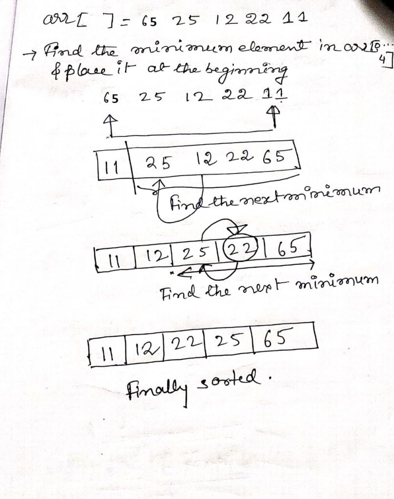
Initially, the sorted sublist is empty and the unsorted sublist is the entire input list. The algorithm proceeds by finding the smallest (or largest, depending on sorting order) element in the unsorted sublist, exchanging (swapping) it with the leftmost unsorted element (putting it in sorted order), and moving the sublist boundaries one element to the right.
The time efficiency of selection sort is quadratic, so there are a number of sorting techniques which have better time complexity than selection sort.
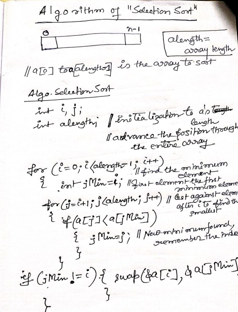
Steps of Selection Sort
- i = 0
- Start with the first element
64as the current minimum. - Compare with elements:
j = 1: Compare64with25,25is smaller.j = 2: Compare25with12,12is smaller.j = 3: Compare12with22,12remains smaller.j = 4: Compare12with11,11is smaller.
- Minimum found at index 4. Swap
64and11. - Array after 1st iteration: 11,25,12,22,64
- Start with the first element
- i = 1
- Start with the second element
25as the current minimum. - Compare with elements:
j = 2: Compare25with12,12is smaller.j = 3: Compare12with22,12remains smaller.j = 4: Compare12with64,12remains smaller.
- Minimum found at index 2. Swap
25and12. - Array after 2nd iteration: 11,12,25,22,6411, 12, 25, 22, 6411,12,25,22,64
- Start with the second element
- i = 2
- Start with the third element
25as the current minimum. - Compare with elements:
j = 3: Compare25with22,22is smaller.j = 4: Compare22with64,22remains smaller.
- Minimum found at index 3. Swap
25and22. - Array after 3rd iteration: 11,12,25,22,64
- Start with the third element
- i = 3
- Start with the fourth element
25as the current minimum. - Compare with elements:
j = 4: Compare25with64,25remains smaller.
- No swap needed since
25is already the minimum. - Array after 4th iteration: 11,12,22,25,64
- Start with the fourth element
- i = 4
- The final element
64is already in its correct place, so no action is needed.
- The final element
Final Sorted Array
11,12,22,25,64
This step-by-step explanation shows how the Selection Sort algorithm works by repeatedly finding the minimum element in the unsorted portion of the array and swapping it with the first unsorted element until the entire array is sorted.
Loop In variants and Insertion Sort
Insertion Sort is a simple sorting algorithm that builds the final sorted array (or list) one item at a time. It is much less efficient on large lists than more advanced algorithms such as quicksort, heapsort, or merge sort.
Here’s the Insertion Sort algorithm.
void insertionSort(int arr[], int n) {
    int i, key, j;
    for (i = 1; i < n; i++) {  // Start with the second element (index 1)
        key = arr[i];          // The element to be inserted into the sorted part
        j = i - 1;             // Index of the previous element

        // Move elements of arr[0..i-1] that are greater than key to one position ahead of their current position
        while (j >= 0 && arr[j] > key) {
            arr[j + 1] = arr[j];
            j = j - 1;
        }
        arr[j + 1] = key;  // Place the key in its correct position
    }
}
Explanation of Each Step
- Initialization:
iis the loop variable that starts from the second element (index 1) because the first element is considered already sorted.keyholds the value of the element to be inserted into the correct position in the sorted portion of the array.jis used to scan through the sorted portion of the array, which is on the left side of the current elementkey.
- Outer Loop (
forloop):
- This loop runs from the second element to the last element (
i = 1ton-1). - Each iteration considers the element
arr[i]as thekeyand tries to insert it into the sorted part of the array on its left side.
- Inner Loop (
whileloop):
- This loop moves elements in the sorted portion of the array (left of
i) that are greater than thekeyone position to the right to make space for thekey. - The loop continues as long as there are elements on the left that are greater than the
keyand as long asjis not negative (indicating the beginning of the array).
- Insert the Key:
- After shifting elements, the correct position for the
keyis found, and it is placed atarr[j + 1].
- End of Outer Loop:
- Once the
forloop completes, the array is fully sorted in ascending order.
Example
For an array arr = [5, 2, 9, 1, 5, 6]:
- 1st iteration (
i=1): Insert2into[5]→[2, 5] - 2nd iteration (
i=2): Insert9into[2, 5]→[2, 5, 9] - 3rd iteration (
i=3): Insert1into[2, 5, 9]→[1, 2, 5, 9] - 4th iteration (
i=4): Insert5into[1, 2, 5, 9]→[1, 2, 5, 5, 9] - 5th iteration (
i=5): Insert6into[1, 2, 5, 5, 9]→[1, 2, 5, 5, 6, 9]
Final sorted array: [1, 2, 5, 5, 6, 9].
Loop Invariant and Proof of Correctness in Insertion Sort
A loop invariant is a condition that holds true before and after each iteration of a loop. It helps in reasoning about the correctness of an algorithm.
For the Insertion Sort algorithm, the loop invariant is:
Invariant: At the start of each iteration of the outer loop (with index i), the subarray arr[0..i-1] consists of the elements that were originally in arr[0..i-1] but in sorted order.
Steps to Prove Correctness
To prove the correctness of the Insertion Sort algorithm using the loop invariant, we must demonstrate three things:
- Initialization: The loop invariant is true before the first iteration.
- Maintenance: If the loop invariant is true before an iteration of the loop, it remains true before the next iteration.
- Termination: When the loop terminates, the loop invariant gives us a useful property that helps prove the algorithm is correct.
1. Initialization
- Before the first iteration (
i = 1), the subarrayarr[0..0]contains only one element (arr[0]), which is trivially sorted. - Therefore, the loop invariant holds true before the first iteration.
2. Maintenance
- Assume that the loop invariant holds at the start of an iteration for
i = k, meaning the subarrayarr[0..k-1]is sorted. - During this iteration, the algorithm selects the element
arr[k](denoted askey) and compares it to the elements in the sorted subarrayarr[0..k-1]. - The inner loop shifts all elements greater than
keyone position to the right, making space forkeyin its correct position. - After placing
keyat the correct position, the subarrayarr[0..k]is sorted. - Hence, the loop invariant holds true at the end of this iteration, ensuring that the subarray
arr[0..k]is sorted.
3. Termination
- The outer loop terminates when
i = n, wherenis the length of the array. - At this point, the loop invariant tells us that the subarray
arr[0..n-1](i.e., the entire array) is sorted. - Therefore, the entire array is sorted when the algorithm completes.
By proving that the loop invariant holds throughout the execution of the loop, we have demonstrated the correctness of the Insertion Sort algorithm. The algorithm sorts the array in ascending order as intended. Let’s analyze the time complexity of the Insertion Sort algorithm step by step. We will examine the time complexity for each part of the algorithm and then sum them up to get the overall time complexity.
Insertion Sort Algorithm (time consumes for each steps)
void insertionSort(int arr[], int n) {
    int i, key, j;

    for (i = 1; i < n; i++) {           // Step 1: Outer loop runs (n-1) times
        key = arr[i];                   // Step 2: Assignment operation (1 time per iteration)
        j = i - 1;                      // Step 3: Assignment operation (1 time per iteration)

        // Step 4: Inner loop - runs while j >= 0 and arr[j] > key
        while (j >= 0 && arr[j] > key) {
            arr[j + 1] = arr[j];        // Step 5: Shifting elements (1 time per shift)
            j = j - 1;                  // Step 6: Decrementing j (1 time per iteration)
        }

        arr[j + 1] = key;               // Step 7: Insertion operation (1 time per iteration)
    }
}
Detailed Time Complexity Analysis
Step 1: Outer Loop (for (i = 1; i < n; i++))
- Time Complexity: The outer loop runs
(n-1)times. Therefore, the time complexity for the outer loop isO(n).
Step 2: Assigning key = arr[i]
- Time Complexity: This is a constant-time operation, and it is executed
(n-1)times (once in each iteration of the outer loop). Therefore, the total time complexity for this step isO(n).
Step 3: Assigning j = i - 1
- Time Complexity: This is also a constant-time operation, executed
(n-1)times. Thus, its total time complexity isO(n).
Step 4: Inner Loop (while (j >= 0 && arr[j] > key))
- Time Complexity:
- In the worst case (reverse sorted array), the inner loop runs
itimes for each iteration of the outer loop. - The first iteration of the outer loop (
i = 1) has the inner loop running1time. - The second iteration (
i = 2) has the inner loop running2times, and so on, up to(n-1)times. - The total number of iterations of the inner loop across all iterations of the outer loop is:
[
1 + 2 + 3 + ……. + (n-1) = n(n-1)/2
] - Therefore, the time complexity for the inner loop in the worst case is
O(n^2).
Step 5: Shifting Elements (arr[j + 1] = arr[j])
- Time Complexity: This operation is performed every time the inner loop condition is met. Therefore, it has the same complexity as the inner loop:
O(n^2)in the worst case.
Step 6: Decrementing j (j = j - 1)
- Time Complexity: This is a constant-time operation, but since it’s part of the inner loop, its total time complexity is
O(n^2)in the worst case.
Step 7: Inserting the key (arr[j + 1] = key)
- Time Complexity: This is a constant-time operation performed once per iteration of the outer loop, giving it a total time complexity of
O(n).
Total Time Complexity
Now, let’s sum up the time complexities of all these steps:
- Outer loop:
O(n) - Assigning
key:O(n) - Assigning
j:O(n) - Inner loop:
O(n^2) - Shifting elements:
O(n^2) - Decrementing
j:O(n^2) - Inserting the
key:O(n)
Overall Time Complexity
The dominant term in this sum is O(n^2) (from the inner loop, shifting elements, and decrementing j). Therefore, the overall time complexity of the Insertion Sort algorithm is: O(n^2) .This is true for the worst case and average case. In the best case, where the array is already sorted, the inner loop doesn’t run, and the overall time complexity reduces to O(n).
Bubble Sort and its analysis
Bubble Sort
Overview
Bubble Sort is one of the simplest sorting algorithms. It works by repeatedly traversing the array, comparing adjacent elements, and swapping them if they are in the wrong order. The process is repeated until the array is completely sorted. Though easy to implement, Bubble Sort is inefficient for large datasets.
Algorithm
Below is the algorithm of Bubble Sort algorithm:
void bubbleSort(int arr[], int n) {
    int i, j, temp;
    for (i = 0; i < n-1; i++) {             // Outer loop for passes
        for (j = 0; j < n-i-1; j++) {       // Inner loop for each pair
            if (arr[j] > arr[j+1]) {        // Compare adjacent elements
                // Swap arr[j] and arr[j+1]
                temp = arr[j];
                arr[j] = arr[j+1];
                arr[j+1] = temp;
            }
        }
    }
}
Explanation
- Initialization:
- The algorithm begins by initializing two loops. The outer loop (
i) runsn-1times, wherenis the number of elements in the array. This ensures that each element is checked and placed in its correct position. - The inner loop (
j) iterates through the array, comparing adjacent elements and swapping them if they are in the wrong order.
- Swapping:
- If the current element
arr[j]is greater than the next elementarr[j+1], they are swapped. The swap is done using a temporary variabletemp.
- Optimization (Optional):
- To optimize, you can add a flag to detect if any swaps were made in an iteration. If no swaps are made, the array is already sorted, and the algorithm can terminate early.
   void bubbleSort(int arr[], int n) {
       int i, j, temp;
       bool swapped;
       for (i = 0; i < n-1; i++) {
           swapped = false;
           for (j = 0; j < n-i-1; j++) {
               if (arr[j] > arr[j+1]) {
                   temp = arr[j];
                   arr[j] = arr[j+1];
                   arr[j+1] = temp;
                   swapped = true;
               }
           }
           if (!swapped) break;  // If no elements were swapped, break
       }
   }
Time Complexity
- Best Case:
- O(n): If the array is already sorted, the inner loop will run without making any swaps. In the optimized version with a swap flag, the algorithm will terminate after the first pass.
- Worst Case:
- O(n^2): This occurs when the array is sorted in reverse order. In this scenario, each element will have to be swapped in every iteration of the inner loop.
- Average Case:
- O(n^2): In general, Bubble Sort will take quadratic time because most elements will need to be swapped as the algorithm progresses.
Space Complexity
- O(1): Bubble Sort is an in-place sorting algorithm, meaning it requires a constant amount of additional memory space regardless of the input size.
Summary
Bubble Sort is an intuitive and easy-to-understand algorithm. However, due to its inefficiency on large datasets, it is rarely used in practice when more efficient sorting algorithms like Quick Sort or Merge Sort are available. Despite its simplicity, it serves as a good introductory algorithm for learning the basics of sorting and algorithm optimization.
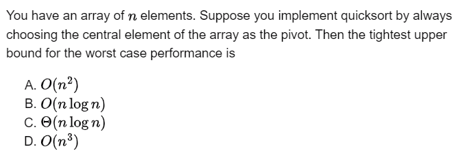
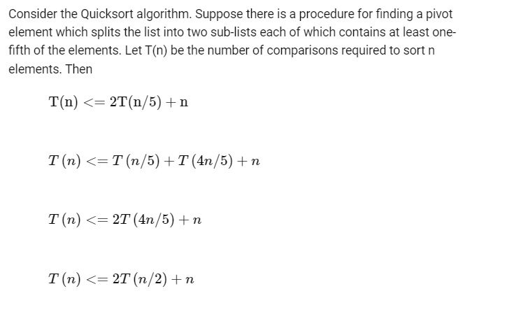
QUICK SORT
Quicksort is an efficient sorting algorithm with a worst-case running time of O(n²) when sorting an array of n numbers. Despite this, quicksort is often the best practical choice due to its average-case performance, with an expected running time of O(n log n) when all elements are distinct. The constant factors in the O(n log n) notation are small, making it more efficient than other algorithms like merge sort. Moreover, quicksort has the advantage of sorting in place, which is particularly useful in virtual memory environments.
Quicksort follows the divide-and-conquer paradigm with three steps:
- Divide: The array is partitioned into two subarrays. Elements smaller than or equal to the pivot are placed in the lower subarray, while those greater than or equal to the pivot are placed in the higher subarray. The pivot’s index is determined during this partitioning.
- Conquer: Quicksort is called recursively on the two subarrays to sort them.
- Combine: No explicit combination is needed since the subarrays are already sorted, making the entire array sorted once the recursion completes.
The algorithm performs well on average, and a randomized version can further improve its performance by reducing the chance of encountering the worst-case scenario. When distinct elements are present, the randomized version ensures a good expected running time, avoiding worst-case behavior.

Partitioning the Array
The key to quicksort is the PARTITION procedure, which rearranges a subarray in place and returns the index that divides the subarray into two parts. The process separates elements into those less than or equal to the pivot and those greater than or equal to the pivot.
In this procedure, the pivot element is always selected as the last element of the subarray, denoted by A[r]. As the algorithm progresses, elements are divided into four distinct regions, though some regions may be empty. These regions represent:
- Elements smaller than or equal to the pivot.
- Elements greater than or equal to the pivot.
- The pivot itself.
- The region yet to be processed.
The properties of these regions are maintained by a loop invariant, ensuring that after each iteration of the loop, the elements are properly partitioned around the pivot.
This process is illustrated with an 8-element array, where PARTITION correctly divides the array by placing the pivot in its correct position and returning the index where the partition occurs.
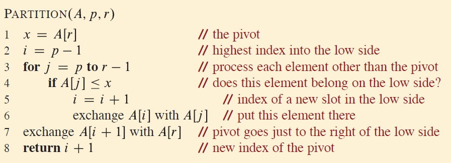
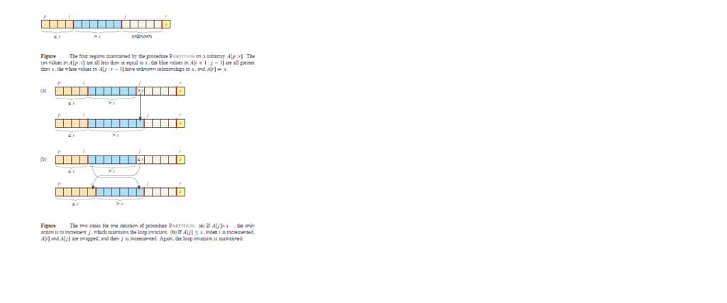
At the beginning of each iteration of the loop in the PARTITION procedure, the following conditions, known as the loop invariant, hold for any index k in the array:
- For
p ≤ k ≤ i: The elements in this region (A[k] ≤ x) are less than or equal to the pivotx. This corresponds to the tan region in below figure. - For
i + 1 ≤ k ≤ j - 1: The elements in this region (A[k] > x) are greater than the pivot. This corresponds to the blue region. - For
k = r: The element at this position (A[k] = x) is equal to the pivot itself. This corresponds to the yellow region.
To ensure the correctness of the algorithm:
- Initialization: Before the first iteration, these conditions hold as the initial regions are set properly, with
iandjindicating the boundaries. - Maintenance: Each iteration of the loop maintains this invariant. During the partitioning process, elements are moved between regions while maintaining the relative order and boundaries set by the loop invariant.
- Termination: When the loop terminates, all elements in the subarray have been processed according to the invariant. At this point, the pivot element is correctly positioned, and the array is partitioned into two regions: elements less than or equal to the pivot on one side, and elements greater than or equal to the pivot on the other.
The correctness of the algorithm follows from this invariant, ensuring that after partitioning, the pivot is in its correct final position.
Initialization:
Before the first iteration of the loop, the indices i = p - 1 and j = p. At this point:
- No values exist between
pandi, and no values lie betweeni + 1andj - 1. Thus, the first two conditions of the loop invariant are trivially satisfied because these regions are empty. - The third condition is satisfied by the assignment made in line 1, which ensures that the pivot is correctly initialized.
Maintenance:
There are two possible outcomes for each iteration, based on the comparison in line 4 of the algorithm:
- Case 1: If
A[j] > x, the loop incrementsj. Since no elements are swapped, the second condition of the loop invariant holds forA[j - 1](the current position ofj), and no other values in the array are affected. - Case 2: If
A[j] ≤ x, the loop incrementsi, swapsA[i]withA[j], and then incrementsj. After the swap:
- The element
A[i]satisfies the first condition (A[i] ≤ x), maintaining the region where elements are less than or equal to the pivot. - The element
A[j - 1](previously swapped) satisfies the second condition (A[j - 1] > x), maintaining the region where elements are greater than the pivot.
This process ensures that the loop invariant holds after each iteration.
Termination:
The loop iterates exactly r - p times, eventually terminating when j = r. At this point, the unexamined subarray from A[j] to A[r - 1] is empty, and every element in the array satisfies one of the three conditions:
- Elements less than or equal to the pivot
x. - Elements greater than
x. - The pivot element itself.
Thus, the array is successfully partitioned into three sets: the low side (less than or equal to x), the high side (greater than x), and the pivot, which is now in its correct position.
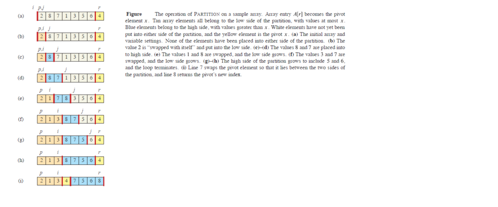
The final two lines of the PARTITION procedure complete the process by swapping the pivot with the leftmost element that is greater than the pivot (x). This operation ensures that the pivot is moved into its correct position in the partitioned array.
After this swap, the pivot is placed in its final sorted position, and the procedure returns the new index of the pivot.
At this point, the output of PARTITION satisfies the requirements of the divide step in quicksort. Specifically:
- All elements to the left of the pivot are less than or equal to the pivot.
- All elements to the right of the pivot are greater than the pivot.
In fact, the partitioning ensures an even stronger condition: after line 3 of QUICKSORT, the element at index q (the pivot) is strictly less than every element in the subarray from q + 1 to r. This guarantees that the pivot is correctly positioned, and the array is properly divided for the recursive steps of quicksort.
Merge Sort
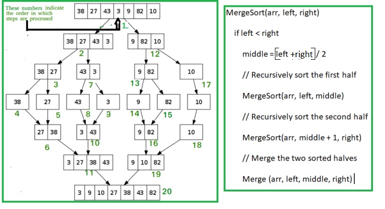
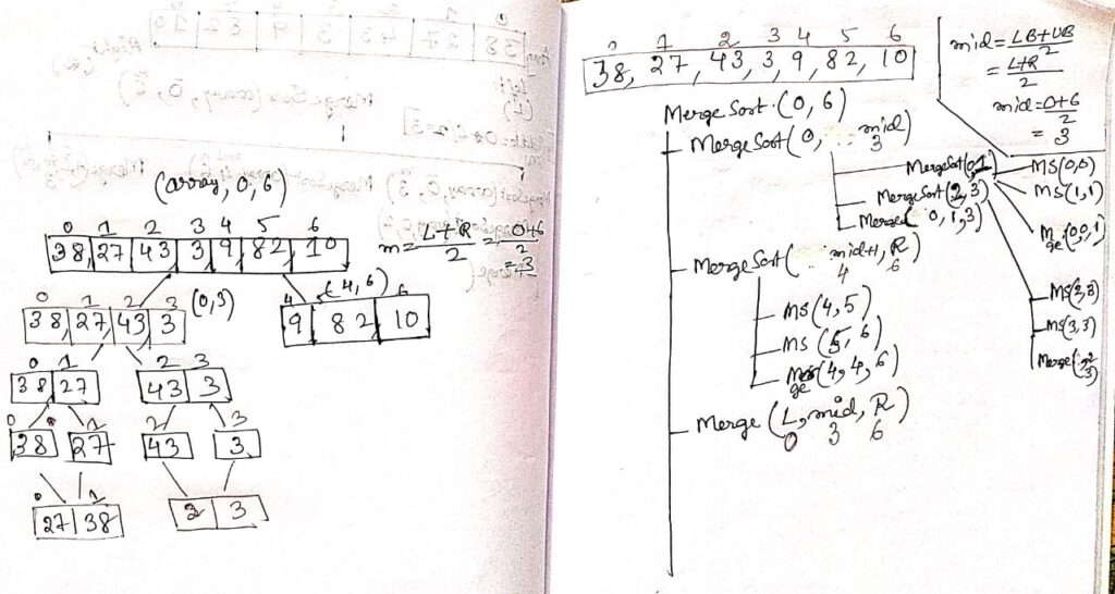
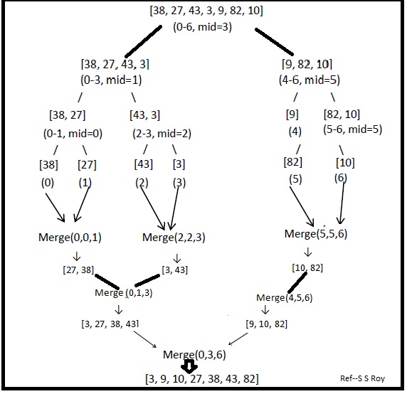
Merge sort is a divide-and-conquer algorithm that recursively splits an array into two halves until each subarray contains only one element, which is considered sorted. It then merges these smaller sorted subarrays back together in a way that results in a sorted array. The merging process compares elements from the two subarrays, placing the smaller element into the result array at each step, and continues until all elements from both subarrays are merged. This process ensures that the entire array is sorted as the subarrays are combined. Merge sort consistently operates with a time complexity of O(n log n), making it efficient for large datasets.
Trees
Binary Trees
A binary tree is a fundamental data structure in computer science, characterized by its hierarchical structure where each node can have a maximum of two children. The term “binary” directly implies that each node in the tree can have zero, one, or two children. This simple yet powerful structure forms the basis for many algorithms and is widely used in various applications such as expression parsing, searching algorithms, and decision-making processes.
What is a Binary Tree?
A binary tree is a collection of nodes arranged in a hierarchy. The topmost node is called the root, and each node contains pointers to its left and right children. If a node has no children, it is called a leaf node. If a node has exactly one child, it is known as a degenerate or skewed node.
For instance, consider the following simple binary tree:
      1
     / \
    2   3
   / \
  4   5
In this binary tree:
- Node 1 is the root with two children (nodes 2 and 3).
- Node 2 has two children (nodes 4 and 5).
- Nodes 3, 4, and 5 are leaf nodes as they do not have any children.
Properties of a Binary Tree
Binary trees have several important properties that are crucial for understanding their structure and behavior:
- Maximum Nodes at Level i: At any level ( i ), the maximum number of nodes that can exist is ( 2^i ). For example, at level 0 (the root level), there can be ( 2^0 = 1 ) node, at level 1 there can be ( 2^1 = 2 ) nodes, and so on.
- Height of the Tree: The height of a binary tree is the length of the longest path from the root to a leaf node. The height determines several other properties of the tree, including its maximum number of nodes and its minimum height.
- Maximum Number of Nodes: The maximum number of nodes in a binary tree of height ( h ) is ( 2^{h+1} – 1 ). This formula accounts for the fact that each level can hold twice as many nodes as the previous level.
- Minimum Height of a Tree: If a binary tree contains ( n ) nodes, its minimum height can be calculated as ( \log_2(n+1) – 1 ).
- Minimum Number of Nodes: Conversely, if a binary tree has a certain height ( h ), the minimum number of nodes it can have is ( h + 1 ). This occurs in a degenerate tree where each node only has one child.
Types of Binary Trees
Binary trees can be classified into several types based on the arrangement and properties of their nodes:
- Full Binary Tree: A binary tree is considered full if every node has either zero or two children. In other words, no node in a full binary tree has only one child. This type of tree is also known as a proper or strict binary tree. Example:
         1
        / \
       2   3
      / \
     4   5
In this example, each node has either two children or none, making it a full binary tree.
- Complete Binary Tree: A complete binary tree is a tree in which all levels are completely filled except possibly the last level, where all nodes are as left as possible. This structure ensures that the tree is as compact as possible, minimizing the tree’s height. Example:
         1
        / \
       2   3
      / \  /
     4   5 6
In this example, the last level is not completely filled, but all nodes are as far left as possible.
- Perfect Binary Tree: A perfect binary tree is a special case of both full and complete binary trees. In a perfect binary tree, all internal nodes have exactly two children, and all leaf nodes are at the same level. Example:
         1
        / \
       2   3
      / \ / \
     4  5 6  7
Here, each node has exactly two children, and all leaf nodes (4, 5, 6, 7) are at the same level.
- Degenerate (or Skewed) Binary Tree: A degenerate binary tree is a tree where each parent node has only one child. This structure effectively reduces the tree to a linked list, leading to inefficient operations compared to a balanced binary tree. Example (Right-Skewed):
   1
    \
     2
      \
       3
        \
         4
Example (Left-Skewed):
       1
      /
     2
    /
   3
  /
4- Balanced Binary Tree: In a balanced binary tree, the difference in height between the left and right subtrees of any node is at most one. Balanced trees ensure that operations such as insertion, deletion, and lookup are performed efficiently. Common examples of balanced binary trees include AVL trees and Red-Black trees. Example:
         1
        / \
       2   3
      /   / \
     4   5   6
Implementation of Binary Trees
Binary trees are commonly implemented using pointers, with each node typically represented as a structure or class containing the data and pointers to its left and right children.
struct node {
    int data;
    struct node *left, *right;
};
In this structure, data represents the value stored in the node, while left and right are pointers to the node’s left and right children, respectively.
Creating a Binary Tree in C
To create a binary tree in C, we typically define a function that recursively constructs the tree by allocating memory for new nodes and assigning their children.
#include<stdio.h>
#include<stdlib.h>

struct node {
    int data;
    struct node *left, *right;
};

struct node* create() {
    struct node *temp;
    int data, choice;
    temp = (struct node *)malloc(sizeof(struct node));

    printf("Press 0 to exit\n");
    printf("Press 1 for new node\n");
    printf("Enter your choice: ");
    scanf("%d", &choice);

    if (choice == 0) {
        return NULL;
    } else {
        printf("Enter the data: ");
        scanf("%d", &data);
        temp->data = data;
        printf("Enter the left child of %d:\n", data);
        temp->left = create();
        printf("Enter the right child of %d:\n", data);
        temp->right = create();
        return temp;
    }
}

int main() {
    struct node *root;
    root = create();
    return 0;
}
In this code, the create function prompts the user to enter data for each node and recursively creates left and right children until the tree is fully constructed.
Tree Traversal Techniques
Traversing a binary tree means visiting each node in a specific order. There are three primary traversal methods:
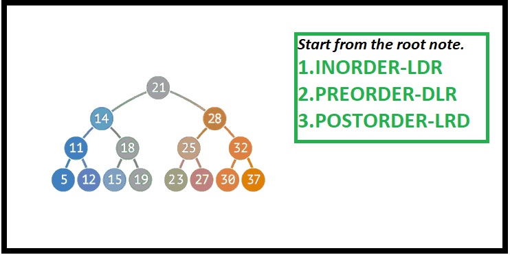
- Inorder Traversal: Visit the left subtree, the root node, and then the right subtree.
- Preorder Traversal: Visit the root node first, followed by the left and right subtrees.
- Postorder Traversal: Visit the left and right subtrees before visiting the root node.
Each traversal technique serves different purposes and can be used depending on the desired outcome of the operation.
Conclusion
Binary trees are a versatile and essential data structure in computer science, providing the foundation for many algorithms and systems. Understanding the properties, types, and implementation of binary trees is crucial for developing efficient solutions in various applications. With balanced trees ensuring optimal performance and different traversal techniques offering flexibility, binary trees remain a cornerstone in the field of data structures.
Here’s a simple C code for creating and traversing a binary tree. The code includes functions to create nodes, insert nodes, and perform inorder, preorder, and postorder traversals.

```c
#include <stdio.h>
#include <stdlib.h>

// Structure for a node in the binary tree
struct Node {
    int data;
    struct Node* left;
    struct Node* right;
};

// Function to create a new node
struct Node* createNode(int data) {
    struct Node* newNode = (struct Node*)malloc(sizeof(struct Node));
    newNode->data = data;
    newNode->left = NULL;
    newNode->right = NULL;
    return newNode;
}

// Function to insert a node in the binary tree
struct Node* insertNode(struct Node* root, int data) {
    if (root == NULL) {
        root = createNode(data);
    } else if (data <= root->data) {
        root->left = insertNode(root->left, data);
    } else {
        root->right = insertNode(root->right, data);
    }
    return root;
}

// Function for Inorder Traversal (Left, Root, Right)
void inorderTraversal(struct Node* root) {
    if (root != NULL) {
        inorderTraversal(root->left);
        printf("%d ", root->data);
        inorderTraversal(root->right);
    }
}

// Function for Preorder Traversal (Root, Left, Right)
void preorderTraversal(struct Node* root) {
    if (root != NULL) {
        printf("%d ", root->data);
        preorderTraversal(root->left);
        preorderTraversal(root->right);
    }
}

// Function for Postorder Traversal (Left, Right, Root)
void postorderTraversal(struct Node* root) {
    if (root != NULL) {
        postorderTraversal(root->left);
        postorderTraversal(root->right);
        printf("%d ", root->data);
    }
}

int main() {
    struct Node* root = NULL;
    int choice, data;

    while (1) {
        printf("\nBinary Tree Operations:\n");
        printf("1. Insert Node\n");
        printf("2. Inorder Traversal\n");
        printf("3. Preorder Traversal\n");
        printf("4. Postorder Traversal\n");
        printf("5. Exit\n");
        printf("Enter your choice: ");
        scanf("%d", &choice);

        switch (choice) {
            case 1:
                printf("Enter data to insert: ");
                scanf("%d", &data);
                root = insertNode(root, data);
                break;
            case 2:
                printf("Inorder Traversal: ");
                inorderTraversal(root);
                printf("\n");
                break;
            case 3:
                printf("Preorder Traversal: ");
                preorderTraversal(root);
                printf("\n");
                break;
            case 4:
                printf("Postorder Traversal: ");
                postorderTraversal(root);
                printf("\n");
                break;
            case 5:
                exit(0);
            default:
                printf("Invalid choice! Please try again.\n");
        }
    }

    return 0;
}
Explanation:
1. createNode(): Allocates memory for a new node and initializes its data, left, and right pointers.
2. insertNode(): Recursively inserts a new node into the binary tree. The new node is inserted based on whether the data is less than or greater than the current node's data.
3. inorderTraversal(): Traverses the tree in inorder sequence (left, root, right).
4. preorderTraversal()**: Traverses the tree in preorder sequence (root, left, right).
5. postorderTraversal()**: Traverses the tree in postorder sequence (left, right, root).
BINARY SEARCH TREE
Level-order traversal
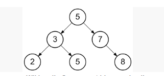
Level-order traversal of a Binary Search Tree (BST) is performed by visiting nodes level by level, starting from the root and moving from left to right across each level.
Example:
Consider the following BST:
       10
      /   \
     6     15
    / \   /  \
   3   8 12   18
Level-Order Traversal Steps:
- Start at the root node (Level 0):
- Visit: 10
- Move to Level 1:
- Visit: 6, 15
- Move to Level 2:
- Visit: 3, 8, 12, 18
Result:
The level-order traversal for the above BST is: 10, 6, 15, 3, 8, 12, 18.
This traversal can be implemented using a queue data structure, where you first enqueue the root, then iteratively dequeue a node, visit it, and enqueue its children.
BST
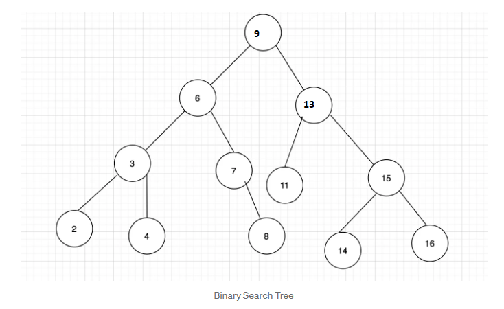
Finding kth smallest element in BST
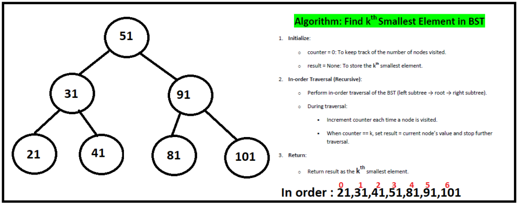
Introduction to AVL Tree
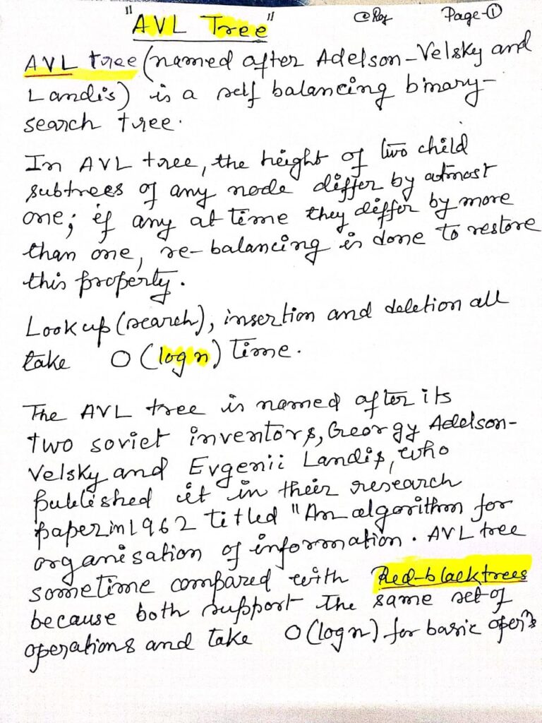
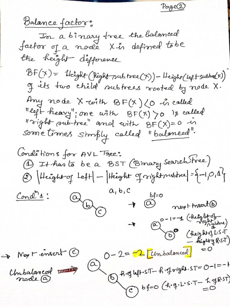
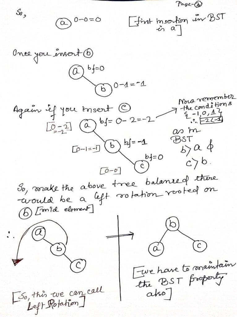
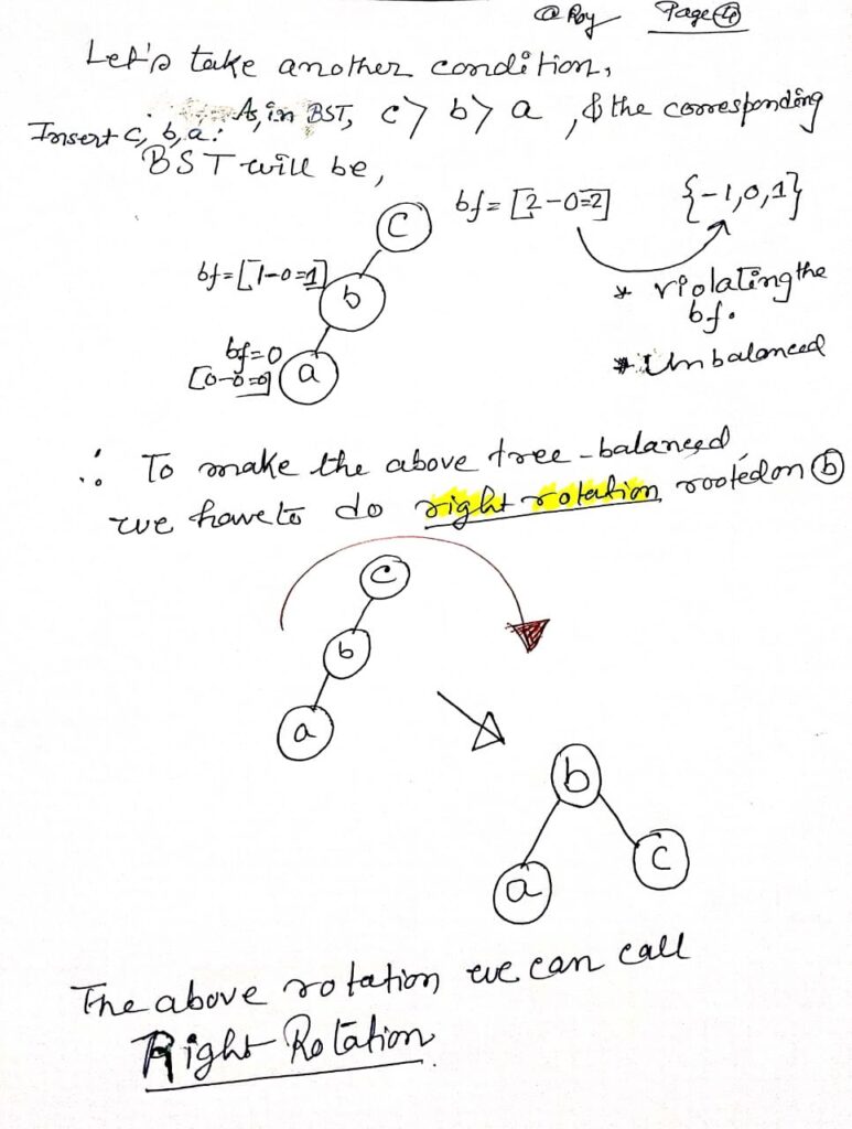
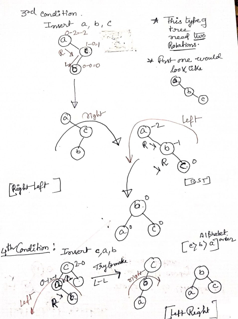
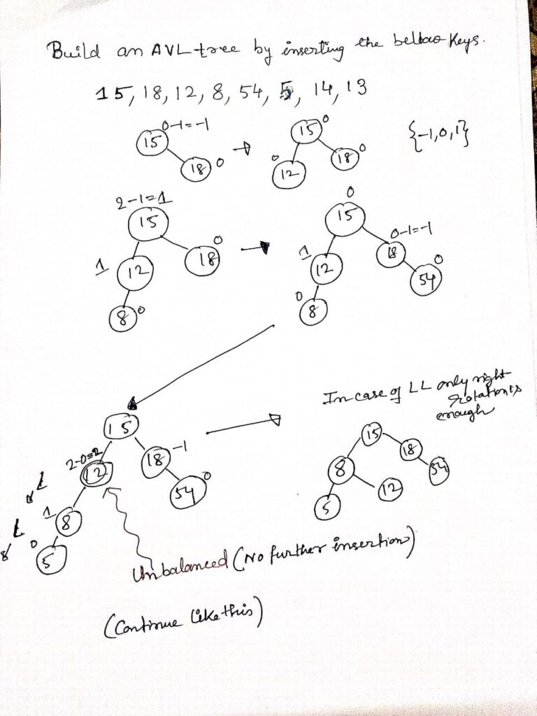
Finding Maximum and Minimum element in a BST
 Algorithm to Find Maximum Element in a Binary Tree
function findMax(root):
    if root is null:
        return null  // Tree is empty

    maxElement = root

    // Traverse to the rightmost node
    while maxElement.right is not null:
        maxElement = maxElement.right

    return maxElement  // Return the maximum element

 Algorithm to Find Minimum Element in a Binary Search Tree

function findMin(root):
    if root is null:
        return null  // Tree is empty

    minElement = root

    // Traverse to the leftmost node
    while minElement.left is not null:
        minElement = minElement.left

    return minElement  // Return the minimum element
Deletion NODEs in AVL Tree
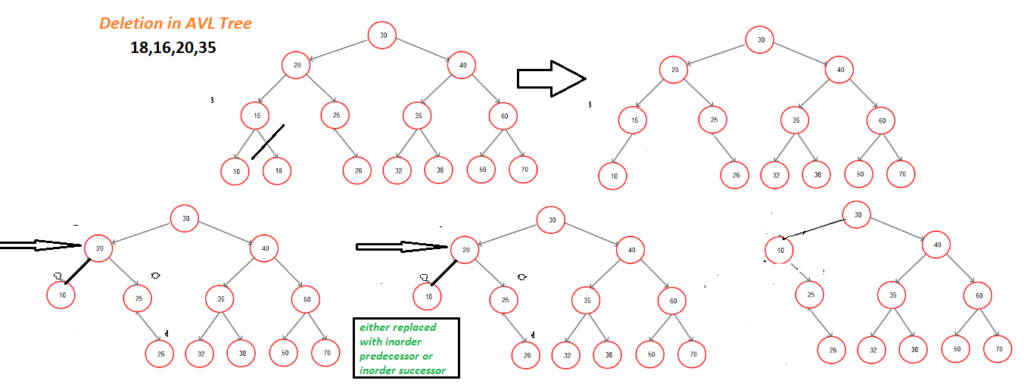
To delete a node in an AVL tree, first, perform a standard Binary Search Tree (BST) deletion: if the node is a leaf, remove it; if it has one child, replace it with its child; if it has two children, find the in-order successor or predecessor, replace the node, . After the deletion, update the balance factors of each ancestor node and rebalance the tree if needed. Rebalancing is done using rotations: Left-Left (LL), Right-Right (RR), Left-Right (LR), or Right-Left (RL), depending on the imbalance detected, ensuring the tree remains balanced.
Hashing
Overview of Hashing
- Hashing is a widely-used method to locate a specific element within a collection of data efficiently.
- It reduces the number of comparisons required for searching.
Benefits of Hashing
Unlike other search approaches:
- Hashing offers exceptional efficiency.
- Its performance is independent of the number of elements present in the dataset.
- Search operations are completed in constant time complexity O(1)O(1).
How Hashing Works
Hash Table
- Hashing uses a specific array-like structure called a hash table to store data.
- Items are placed in the hash table based on a calculated hash key value.
Hash Key Value
- A hash key value is a unique identifier that determines the storage location of an item in the hash table.
- It is derived using a mathematical hash function.
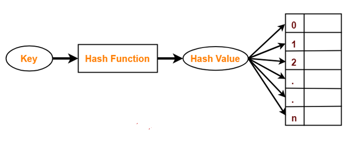
Hash Function
- The hash function takes a data item as input and produces a small integer output, referred to as the hash value.
- The hash value serves as the index to store the data in the hash table.
Types of Hash Functions
Common types of hash functions include:
- Mid-Square Method
- Division Method
- Folding Method
The choice of hash function depends on the user’s requirements.
Features of a Good Hash Function
A well-designed hash function has the following characteristics:
- It is computationally efficient.
- It minimizes collisions (where two keys map to the same index).
- It ensures an even distribution of keys across the hash table.
Searching Techniques Comparison
Traditional searching methods, such as linear search, binary search, or search trees, rely on the size of the dataset, which affects their time complexity:
- Linear Search: O(n)O(n) for unsorted arrays of size nn.
- Binary Search: O(logn)O(\log n) for sorted arrays or binary search trees.
Drawbacks of Traditional Methods
- As the dataset grows, the time taken to search increases significantly.
- This becomes a challenge for large-scale datasets.
Example of Hashing: Separate Chaining
Problem Statement
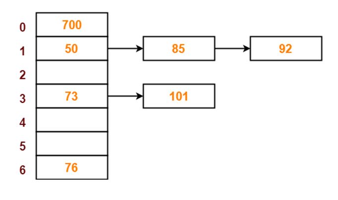
Using the hash function key mod 7, insert the following sequence into a hash table:
50,700,76,85,92,73,10150, 700, 76, 85, 92, 73, 101
Use separate chaining to handle collisions.
Solution Steps
- Initialize the Hash Table
- The hash table should have 7 buckets (hash values range from 0 to 6).
- Insert Items
- Calculate the hash value for each key:
- Key 50: 50mod 7=50 mod 7 = 1, stored in bucket 1.
- Key 700: 700mod 7=0700 mod 7 = 0, stored in bucket 0.
- Key 76: 76mod 7=76 mod 7 = 6, stored in bucket 6.
- Key 85: 85mod 7=85 mod 7 = 1, causing a collision. Add to bucket 1 using a linked list.
- Continue similarly for keys 92,73,92, 73, and 101, using linked lists where collisions occur.
- Calculate the hash value for each key:
Alternative Method: Open Addressing
What is Open Addressing?
- In this method, all data is stored directly within the hash table.
- Unlike separate chaining, no external structures are used.
Techniques in Open Addressing
- Linear Probing: Sequentially checks the next bucket for empty space.
- Pros: Easy to implement.
- Cons: Suffers from clustering.
- Quadratic Probing: Jumps to the i2i^2-th bucket in the ii-th iteration to resolve collisions.
- Double Hashing: Applies a second hash function to determine the next bucket in case of a collision.
Operations in Open Addressing
Insertion
- Compute the hash value for the key.
- If a collision occurs, probe according to the technique until an empty bucket is found.
Searching
- Calculate the hash value and inspect the corresponding bucket.
- Continue probing if the bucket does not contain the desired key until the key or an empty bucket is found.
Deletion
- Locate the key and remove it. Mark the bucket as “deleted.”
- Deleted buckets are reused during insertion but not skipped during searches.
Summary of Open Addressing Techniques
| Feature | Linear Probing | Quadratic Probing | Double Hashing |
| Primary Clustering | Yes | No | No |
| Secondary Clustering | Yes | Yes | No |
| Cache Performance | Best | Moderate | Poor |
Load Factor (α\alpha) in Open Addressing
- Load factor is the ratio of the number of stored elements to the total size of the table.
- For open addressing, α\alpha lies between 0 and 1.
Why?
- All data is stored within the hash table, so the table size is always sufficient for the stored items.
Practice Problem: Linear Probing
Using the hash function key mod 7, insert the following keys:
50,700,76,85,92,73,10150, 700, 76, 85, 92, 73, 101
Resolve collisions using linear probing.