- Introduction to Analytics –
- Business Analytics , Models-Predictive, Descriptive, & Decision Models(AprioriAlgorithm),
- Analytical Techniques
- Data Prep & Tuning–
- Data Transformations (Single & Multiple Predictors)
- Handling Missing Values (Removal, Imputation, Binning) Model Tuning, Data Splitting & Resampling
Predictive Modeling –
Propensity, Cluster, & Collaborative Filtering Models, Statistical Modeling
Regression Model Comparison –
Linear(Fitting a st line using the least square method), Measurement of metrics(Linear Regression),Multiple Linear Regression, Logistic Regression & Non-Linear Regression
Regression Trees & Rules
- Classification Model Comparison– Classification Model Performance – Linear(Support Vector Machine-SVM & Non-Linear Classification(SVM-Non Linear)(NN-Part-A & NN-Part-B, Backpropagation, Classification Trees(Decision Tree ; C4.5 & Rules- Model Evaluation(Classification)
- Addressing Class Imbalance – Impact of Class Imbalance, Model Tuning & Adjustments Sampling Methods * Cost-Sensitive Training * Predictor Importance & Model Performance Factors. Time Series Analysis
AprioriAlgorithm
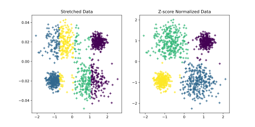
VARIOUS NORMALIZATION TECHNIQUES
Transformations to Resolve Skewness
Dealing with Missing Values
In many situations, certain predictors lack values for specific samples. These missing values might be structurally missing, such as the number of children a man has biologically given birth to. Alternatively, some data points might be unavailable or were not recorded during the model development phase. Understanding the reasons behind missing values is crucial. The first step is to determine whether the missing data pattern is connected to the outcome. This phenomenon, known as “informative missingness,” implies that the absence of data itself carries meaningful insights. Such informative missingness can introduce substantial bias into the model. For instance, an earlier example discussed predicting a patient’s response to a drug. If the drug is highly ineffective or causes severe side effects, patients may skip doctor visits or withdraw from the study. Here, the likelihood of missing values is directly linked to the treatment’s impact.
Informative missingness is also evident in customer ratings, where individuals are more likely to provide feedback when they hold strong opinions—whether positive or negative. This often leads to a polarized dataset, with few ratings falling in the middle range. A notable instance of this occurred during the Netflix Prize competition, where participants aimed to predict user preferences for movies based on prior ratings. The “Napoleon Dynamite Effect” posed challenges for many competitors, as individuals who rated the movie tended to either love it or hate it, creating a highly skewed dataset.
It is important to distinguish between missing data and censored data, as the two are not the same. Censored data refers to situations where the exact value is unknown, but some information about it is still available. For instance, a company that rents DVDs by mail might include the duration a customer keeps a movie in its models. If the movie has not been returned, the exact time cannot be determined, but it is known to be at least as long as the current duration. Similarly, censored data is common in laboratory measurements, where certain tests cannot detect values below a specific threshold. In these cases, it is clear the value is less than the detection limit, but its precise amount remains unmeasured.
How are censored data handled differently from missing data? In traditional statistical modeling aimed at interpretation or inference, censoring is typically addressed formally by making assumptions about the underlying mechanism. However, in predictive modeling, censored data are often treated as if they were simply missing, or the censored value itself is used as a substitute. For example, when a measurement falls below the detection limit, the limit value may be used as a stand-in for the actual measurement. Alternatively, a random value between zero and the detection limit might be assigned to represent the censored data.
There are cases where the missing values might be concentrated in specific samples. For large data sets, removal of samples based on missing values is not a problem, assuming that the missingness is not informative. In smaller data sets, there is a steep price in removing samples; some of the alternative approaches described below may be more appropriate. If we do not remove the missing data, there are two general approaches. First, a few predictive models, especially tree-based techniques, can specifically account for missing data. Alternatively, missing data can be imputed. In this case, we can use information in the training set predictors to, in essence, estimate the values of other predictors. This amounts to a predictive model within a predictive model.
Imputation has been widely explored in statistical research, primarily in the context of developing accurate hypothesis testing procedures when faced with missing data. However, this differs from the objectives of predictive modeling, where the focus is on improving prediction accuracy rather than ensuring valid inferences. Research specifically addressing imputation in predictive models is relatively limited. For instance, Saar-Tsechansky and Provost (2007b) investigated how different models handle missing values, while Jerez et al. (2010) examined various imputation techniques for a specific dataset.
As previously mentioned, imputation adds an extra layer of modeling, where missing values in predictors are estimated based on information from other predictors. A typical method involves creating an imputation model for each predictor using the training set. Before training the primary model or making predictions on new data, these imputation models are used to fill in missing values. It is important to acknowledge that this additional layer of modeling introduces uncertainty. When resampling techniques are employed to select tuning parameters or assess performance, it is essential to incorporate the imputation process within the resampling framework. While this approach increases the computational demands of model building, it provides more accurate performance estimates.
If only a few predictors are affected by missing values, an exploratory analysis to investigate relationships among predictors can be advantageous. Techniques such as visualization or PCA can help uncover strong correlations between variables. For predictors with missing values that are closely correlated with those having few missing values, a focused imputation model can often produce effective outcomes, as demonstrated in the example below.
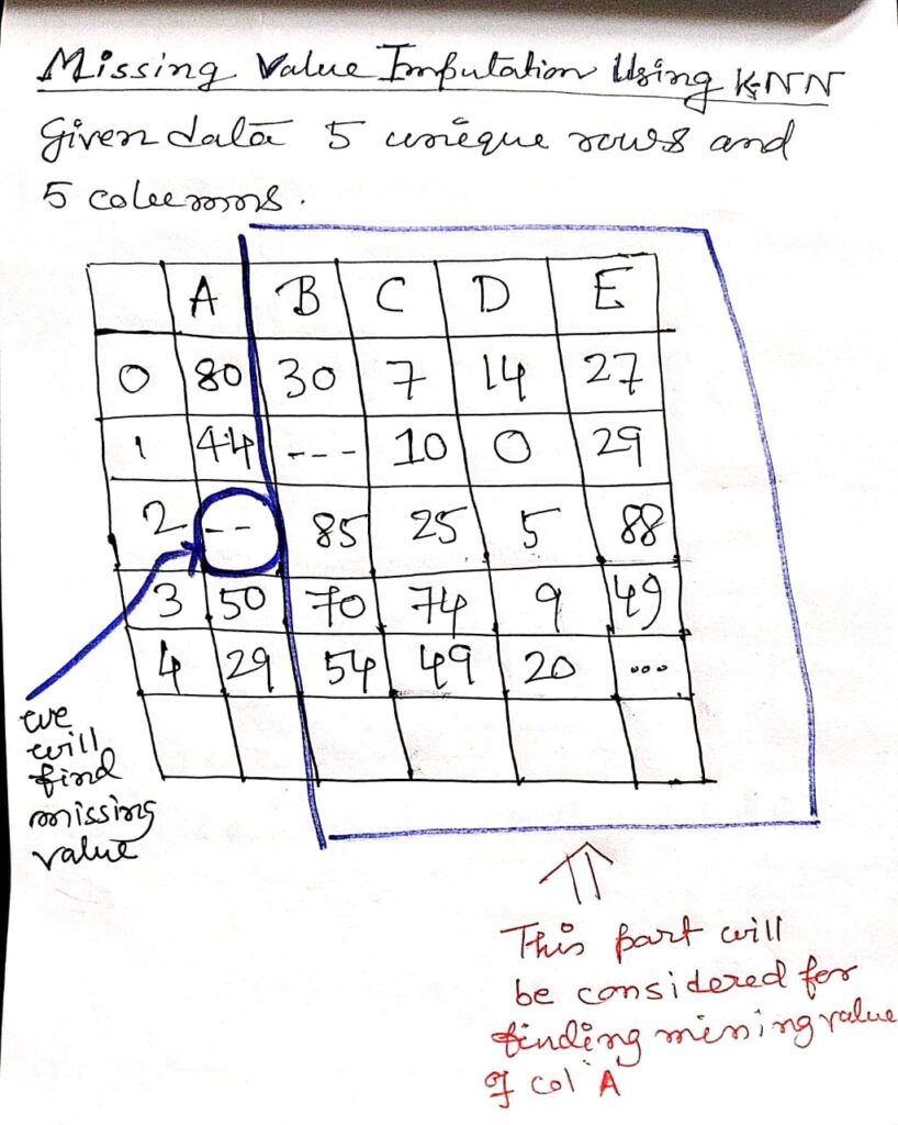
A commonly used method for imputation is the K-nearest neighbor (KNN) model. In this approach, missing values for a new sample are estimated by identifying the samples in the training set that are “closest” to it and averaging the values of these neighboring points to fill in the missing data. Troyanskaya et al. (2001) explored this method, particularly for high-dimensional datasets with small sample sizes.
One advantage of the KNN approach is that the imputed values remain within the range of the training set, preserving the data’s original scale. However, a notable drawback is the need to reference the entire training set each time a missing value is imputed, which can be computationally demanding. Additionally, this method requires tuning key parameters, such as the number of neighbors and the technique used to determine proximity.
The determination of “closeness” between two points is another important aspect of the K-nearest neighbor method. However, Troyanskaya et al. (2001) observed that the nearest neighbor technique demonstrates considerable robustness to variations in these tuning parameters and the proportion of missing data.
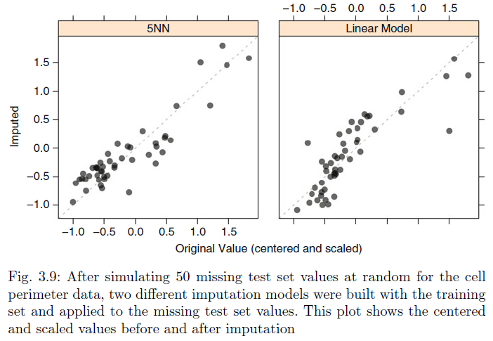
A predictor measuring cell perimeter was previously used to illustrate skewness. To demonstrate the K-nearest neighbor method, a 5-nearest neighbor model was built using the training set values. Missing values were artificially introduced into 50 test set cell perimeter values, which were subsequently imputed using this model. The results are displayed in the left-hand panel of above Fig, where the scatter plot illustrates the imputation’s effectiveness. The model achieved a high correlation of 0.91 between the actual and imputed values, indicating strong predictive performance. Alternatively, a simpler strategy can be applied for imputing cell perimeter values. Cell fiber length, another predictor related to cell size, has a very high correlation (0.99) with cell perimeter data. By employing a straightforward linear regression model, it is possible to predict the missing values. The results of this method are shown in the right-hand panel of above Fig. where the correlation between actual and imputed values is 0.85.
Here’s a simple example of how to handle missing values in Python using the popular pandas library. In this example, we will create a dataset with missing values and then handle them using imputation (filling missing values with the mean of the column).
Step-by-Step Example:
- Create a DataFrame with missing values.
- Impute missing values by filling them with the mean of the respective columns
import pandas as pd

# Step 1: Create a DataFrame with missing values
data = {
    'Name': ['Alice', 'Bob', 'Charlie', 'David', 'Eva'],
    'Age': [25, None, 30, None, 22],
    'Salary': [50000, 60000, None, 55000, 70000]
}

df = pd.DataFrame(data)

print("Original DataFrame with missing values:")
print(df)

# Step 2: Impute missing values with the mean of each column
df['Age'].fillna(df['Age'].mean(), inplace=True)
df['Salary'].fillna(df['Salary'].mean(), inplace=True)

print("\nDataFrame after imputation:")
print(df)

Original DataFrame with missing values:
      Name   Age   Salary
0    Alice  25.0  50000.0
1      Bob   NaN  60000.0
2  Charlie  30.0      NaN
3    David   NaN  55000.0
4      Eva  22.0  70000.0

DataFrame after imputation:
      Name   Age   Salary
0    Alice  25.0  50000.0
1      Bob  26.75  60000.0
2  Charlie  30.0  61250.0
3    David  26.75  55000.0
4      Eva  22.0  70000.0
Explanation:
- Creating the DataFrame: The
AgeandSalarycolumns have some missing values (NaN). - Imputation: The missing values in
Ageare filled with the column’s mean (26.75), and the missing values inSalaryare filled with the mean of that column (61250).
Here’s an extended version of the Python code with additional methods for handling missing values, including:
- Imputation using Mean, Median, and Mode.
- Dropping rows or columns with missing values.
- Filling missing values with forward-fill or backward-fill.
import pandas as pd

# Step 1: Create a DataFrame with missing values
data = {
    'Name': ['Alice', 'Bob', 'Charlie', 'David', 'Eva'],
    'Age': [25, None, 30, None, 22],
    'Salary': [50000, 60000, None, 55000, 70000],
    'Department': ['HR', None, 'Engineering', 'Marketing', 'Finance']
}

df = pd.DataFrame(data)

print("Original DataFrame with missing values:")
print(df)

# Step 2: Impute missing values with different strategies

# Impute missing values in the 'Age' column with the mean
df['Age'].fillna(df['Age'].mean(), inplace=True)
print("\nDataFrame after filling missing 'Age' with mean:")
print(df)

# Impute missing values in the 'Salary' column with the median
df['Salary'].fillna(df['Salary'].median(), inplace=True)
print("\nDataFrame after filling missing 'Salary' with median:")
print(df)

# Impute missing values in the 'Department' column with the mode (most frequent value)
df['Department'].fillna(df['Department'].mode()[0], inplace=True)
print("\nDataFrame after filling missing 'Department' with mode:")
print(df)

# Step 3: Drop rows with missing values
df_dropped_rows = df.dropna()
print("\nDataFrame after dropping rows with missing values:")
print(df_dropped_rows)

# Step 4: Drop columns with missing values
df_dropped_columns = df.dropna(axis=1)
print("\nDataFrame after dropping columns with missing values:")
print(df_dropped_columns)

# Step 5: Forward-fill (propagate last valid value)
df_forward_fill = df.fillna(method='ffill')
print("\nDataFrame after forward-filling missing values:")
print(df_forward_fill)

# Step 6: Backward-fill (use next valid value)
df_backward_fill = df.fillna(method='bfill')
print("\nDataFrame after backward-filling missing values:")
print(df_backward_fill)
Output :
Original DataFrame with missing values:
      Name   Age   Salary   Department
0    Alice  25.0  50000.0          HR
1      Bob   NaN  60000.0         None
2  Charlie  30.0      NaN  Engineering
3    David   NaN  55000.0    Marketing
4      Eva  22.0  70000.0      Finance

DataFrame after filling missing 'Age' with mean:
      Name   Age   Salary   Department
0    Alice  25.0  50000.0          HR
1      Bob  26.75  60000.0         None
2  Charlie  30.0      NaN  Engineering
3    David  26.75  55000.0    Marketing
4      Eva  22.0  70000.0      Finance

DataFrame after filling missing 'Salary' with median:
      Name   Age   Salary   Department
0    Alice  25.0  50000.0          HR
1      Bob  26.75  60000.0         None
2  Charlie  30.0  61250.0  Engineering
3    David  26.75  55000.0    Marketing
4      Eva  22.0  70000.0      Finance

DataFrame after filling missing 'Department' with mode:
      Name   Age   Salary   Department
0    Alice  25.0  50000.0          HR
1      Bob  26.75  60000.0          HR
2  Charlie  30.0  61250.0  Engineering
3    David  26.75  55000.0    Marketing
4      Eva  22.0  70000.0      Finance

DataFrame after dropping rows with missing values:
      Name   Age   Salary   Department
0    Alice  25.0  50000.0          HR
2  Charlie  30.0  61250.0  Engineering
4      Eva  22.0  70000.0      Finance

DataFrame after dropping columns with missing values:
      Name
0    Alice
1      Bob
2  Charlie
3    David
4      Eva

DataFrame after forward-filling missing values:
      Name   Age   Salary   Department
0    Alice  25.0  50000.0          HR
1      Bob  26.75  60000.0          HR
2  Charlie  30.0  61250.0  Engineering
3    David  26.75  55000.0    Marketing
4      Eva  22.0  70000.0      Finance

DataFrame after backward-filling missing values:
      Name   Age   Salary   Department
0    Alice  25.0  50000.0          HR
1      Bob  26.75  60000.0  Engineering
2  Charlie  30.0  61250.0  Engineering
3    David  26.75  55000.0    Marketing
4      Eva  22.0  70000.0      Finance
Explanation of Additions:
- Filling with Mean, Median, and Mode: Missing values in
Age,Salary, andDepartmentare filled with the mean, median, and mode of their respective columns, respectively. - Dropping Rows or Columns: Rows or columns containing missing values are removed using the
dropna()method. - Forward-fill and Backward-fill: The
fillna(method='ffill')method propagates the last valid value to fill in the missing values, whilefillna(method='bfill')uses the next valid value.
Removing predictors before model training can provide multiple benefits. Firstly, a reduction in the number of predictors reduces both the computational cost and the complexity of the model, making it faster and more efficient to train.
Removing Predictors
Secondly, when two predictors are highly correlated, it suggests they are capturing similar underlying information. In such cases, removing one predictor should not harm the model’s performance but might lead to a simpler and more interpretable model.
Thirdly, certain models might struggle with predictors exhibiting degenerate distributions or those with only a few unique values. In these situations, removing these predictors can lead to improved model stability and performance.
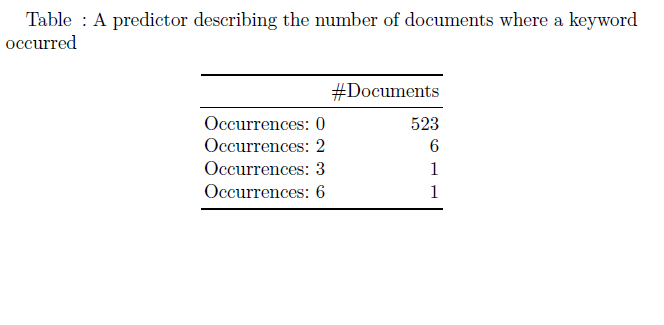
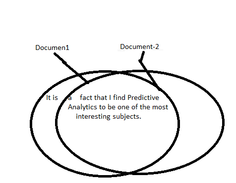
For example, consider a predictor variable that describes the frequency of keyword occurrences across several documents. In a dataset with 531 documents, most of the documents (523) do not contain the keyword, while only a small number have a few occurrences. Such a variable would have little impact on certain models, like tree-based models, which would ignore it during splits. However, models like linear regression could face issues with these kinds of predictors due to computational difficulties. In these cases, the uninformative variable can be safely removed.
Moreover, some predictors may have only a small number of unique values that occur infrequently. These “near-zero variance predictors” might have a dominant value in most cases, but very few other values, which can disproportionately influence the model.
In scenarios such as text mining, where keyword counts are recorded across a large number of documents, predictors with very low variance could be problematic. For example, a keyword might appear in only a few documents, leading to an imbalanced distribution of values. A potential distribution could look like this: of 531 documents, 523 have zero occurrences of the keyword, 6 documents have two occurrences, and only 1 or 2 documents contain more. This type of distribution is often skewed, where one value occurs much more frequently than others, resulting in an imbalance that could negatively affect model performance.
To detect near-zero variance predictors, it’s crucial to check the proportion of unique values relative to the sample size. In the document example, only four unique counts exist across 531 documents, which results in 0.8% unique values. Although a small percentage of unique values in itself may not be an issue, the disproportionate frequency of certain values can signal that the predictor is unhelpful. A rule of thumb for diagnosing such issues is to examine the ratio of the most frequent value’s occurrences to the second most frequent. If this ratio is too large, the predictor is likely to be near-zero variance.
By detecting and removing such predictors, the model can be made more efficient, reducing the risk of overfitting and improving interpretability. Additionally, this approach helps avoid numerical issues in certain models that are sensitive to degenerate predictors.
The fraction of unique values over the sample size is low (say 10 %).
• The ratio of the frequency of the most prevalent value to the frequency of the second most prevalent value is large (say around 20). If both of these criteria are true and the model in question is susceptible to this type of predictor, it may be advantageous to remove the variable from the model.
Between-Predictor Correlations
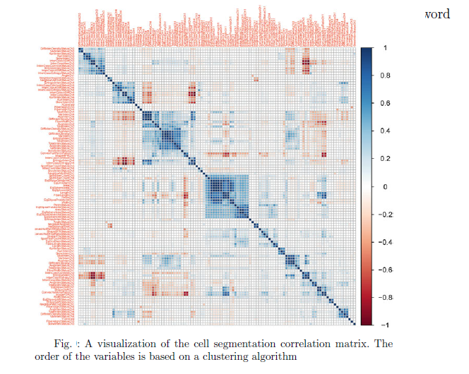
Collinearity refers to a situation where predictor variables are highly correlated. When multiple predictors show strong correlations, it’s known as multicollinearity. For instance, in cell segmentation data, predictors like cell perimeter, width, and length are correlated, reflecting cell size and morphology (e.g., roughness).
A correlation matrix visually shows the strength of pairwise correlations, with dark blue indicating strong positive correlations, dark red for negative correlations, and white for no relationship. Grouping collinear predictors using clustering techniques helps identify correlated clusters.
If many predictors make visual inspection difficult, techniques like PCA can highlight major correlations, such as when the first principal component captures most of the variance, indicating redundancy in predictors.
Reference: Kuhn, M. “Applied predictive modeling.” (2013). Page No : 45-47
🔍 Between-Predictor Heuristic Approach
Missing Value Imputation by KNN


Data Splitting by InterQuartile Range(IQR)
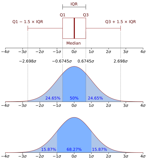
By Jhguch at en.wikipedia, CC BY-SA 2.5, https://commons.wikimedia.org/w/index.php?curid=14524285
These quartiles are denoted by Q1 (also called the lower quartile), Q2 (the median), and Q3 (also called the upper quartile).
Principal Component Analysis
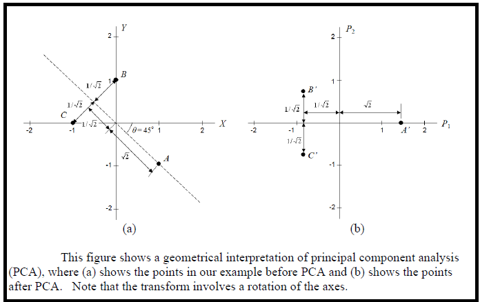
Solved Examples : PCA
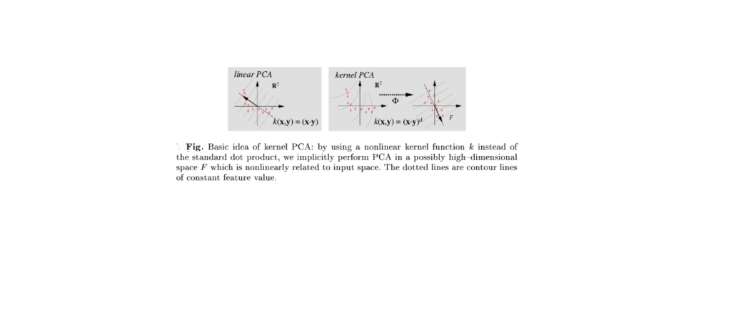
PCA with Kernel
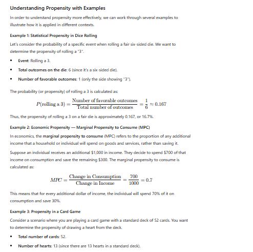
Propensity: Concept and Application
Definition of Propensity
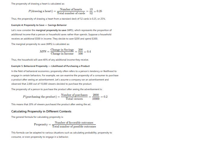
Propensity refers to an inherent tendency or likelihood of something happening, generally related to the probability of a particular event occurring. The term is commonly used in statistics, economics, psychology, and various other disciplines to describe the tendency or probability that a certain outcome or event will happen given certain conditions or factors. In the realm of probability and statistics, propensity is often used to refer to the expected behavior or outcome based on a series of probabilities and conditions.
In other words, propensity can be thought of as a measure of how likely an event is to occur under a specific set of circumstances.
Types of Propensity
- Statistical Propensity: This type refers to the probability that an event will occur given certain data or information. It involves calculating the likelihood of events based on historical or observed data.
- Economic Propensity: In economics, the term “propensity” is often used to refer to the “marginal propensity,” which is the likelihood that an individual or household will spend or save additional income.
- Behavioral Propensity: In psychology and behavioral economics, propensity refers to an individual’s inclination or tendency to perform a particular action or decision.

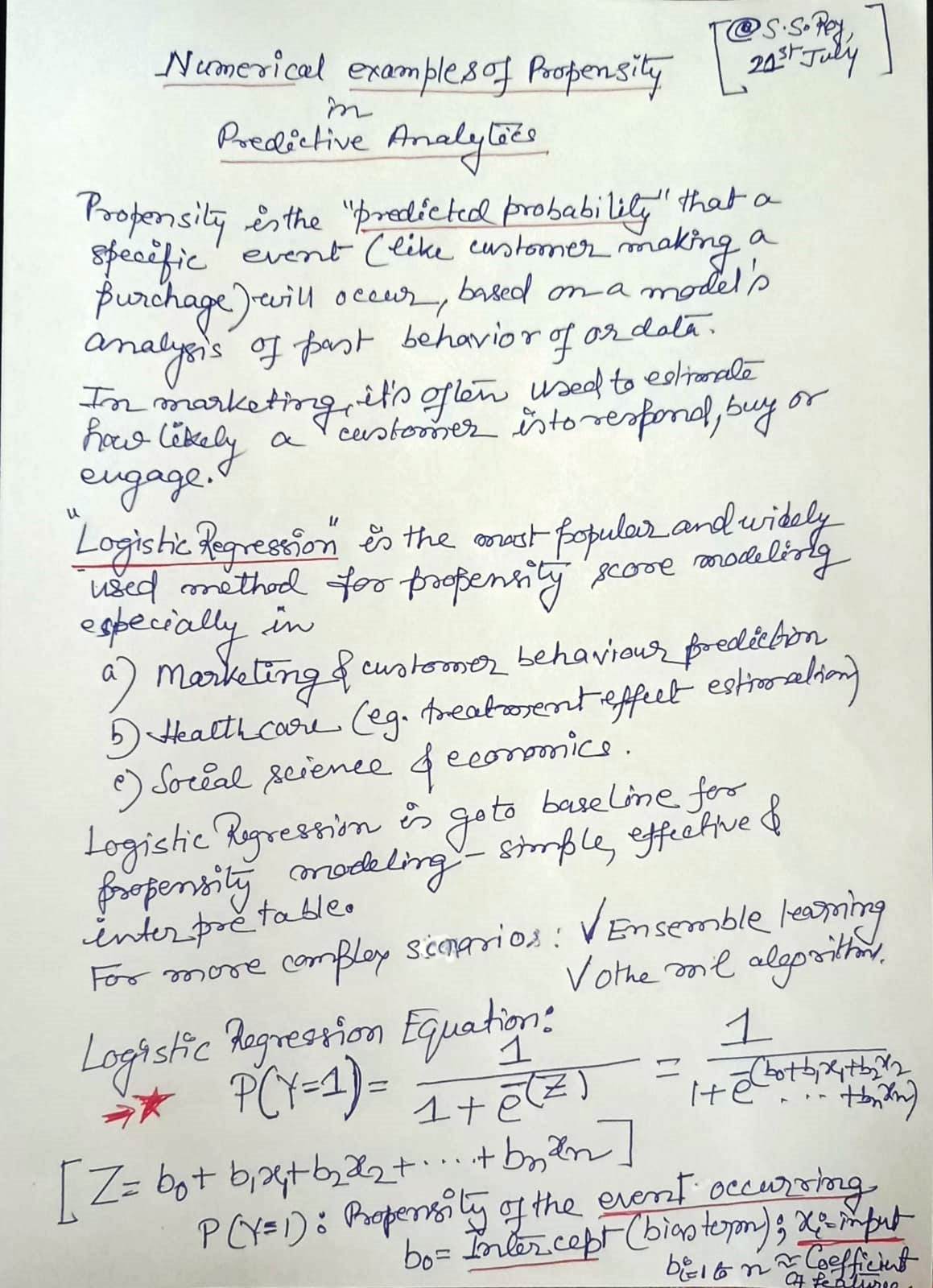
Propensity in Predictive Modeling
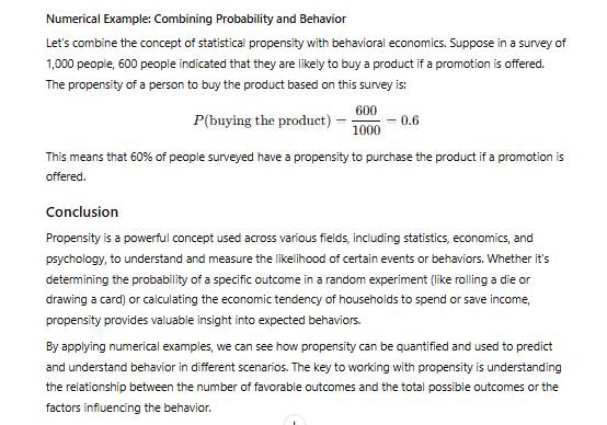
In machine learning, propensity models are used to predict the likelihood or probability that a specific event will occur. For instance, in marketing, a propensity model can predict the likelihood that a customer will purchase a product or respond to a marketing campaign. These models are built using data from previous interactions, customer behavior, demographics, and other relevant factors. The goal is to understand how different features of the data contribute to the likelihood of an event.
For example, in an e-commerce setting, a propensity model might predict the likelihood that a user will purchase a specific item based on their browsing history, search queries, and past purchases. This allows businesses to target their marketing strategies more effectively, improving conversion rates and customer satisfaction.
Key Applications of Propensity in Machine Learning
- Customer Churn Prediction: One of the most important uses of propensity in machine learning is predicting customer churn, which refers to the likelihood that a customer will stop using a service or product. By analyzing historical data, such as past customer interactions, purchases, usage patterns, and engagement, machine learning models can calculate the propensity of a customer to churn. By identifying customers with a high propensity to churn, businesses can take proactive steps to retain them, such as offering personalized promotions or targeted communication.
- Targeted Marketing and Personalization: Propensity models are widely used in marketing to predict the likelihood of a customer engaging with a particular campaign, responding to a promotional offer, or making a purchase. For example, a retailer may use a propensity model to predict the likelihood of a customer responding to a discount offer for a particular product. This allows the retailer to focus their efforts on the customers with the highest propensity, improving the efficiency of their marketing strategies and increasing return on investment (ROI).
- Recommendation Systems: Propensity also plays a crucial role in recommendation systems, where the goal is to predict the likelihood of a user engaging with a product, service, or content. For example, in a movie recommendation system, the model might predict the propensity of a user to enjoy and watch a particular movie based on their past preferences and ratings. By calculating these propensities, the system can recommend the most relevant items to users, improving user experience and engagement.
- Fraud Detection: In financial services, propensity models are used to predict the likelihood that a transaction or activity is fraudulent. By analyzing transaction patterns, user behavior, and historical data, machine learning models can estimate the propensity of a given action to be fraudulent. This helps in flagging high-risk transactions and protecting users from potential financial losses.
Techniques for Propensity Modeling
Several machine learning techniques are used for propensity modeling, with some of the most common methods being:
- Logistic Regression: A popular method for predicting binary outcomes, logistic regression models the probability of an event occurring by using a sigmoid function to output values between 0 and 1, which can be interpreted as the propensity of an event.
- Decision Trees and Random Forests: Decision trees can be used to segment the data based on different features, and each leaf node represents a predicted propensity for an event. Random forests combine multiple decision trees to improve prediction accuracy.
- Gradient Boosting: Gradient boosting methods such as XGBoost or LightGBM can be used to build more accurate propensity models by combining weak learners to form a strong predictive model.
- Neural Networks: Deep learning techniques, especially in the form of neural networks, can be used for complex propensity modeling, especially when dealing with large datasets with intricate relationships between features.
Evaluation of Propensity Models
To assess the effectiveness of propensity models, various performance metrics are used. These include:
- Accuracy: Measures how often the model’s predictions are correct.
- AUC-ROC (Area Under the Receiver Operating Characteristic Curve): This metric evaluates the tradeoff between true positive rate and false positive rate, providing a comprehensive view of the model’s ability to distinguish between different classes (such as ‘purchase’ vs ‘no purchase’).
- Precision and Recall: Precision measures how many of the predicted positive cases are actually positive, while recall measures how many of the actual positive cases are identified by the model. These metrics are especially useful in situations where false positives or false negatives have different implications (e.g., in fraud detection or medical diagnosis).
Conclusion
In machine learning, propensity is a fundamental concept that helps in predicting the likelihood of specific events based on data patterns. Propensity models enable businesses to make informed decisions, such as targeting the right customers for marketing campaigns, predicting customer churn, or recommending personalized content. By leveraging techniques like logistic regression, decision trees, and gradient boosting, machine learning models can calculate propensities that enhance decision-making and improve outcomes. As machine learning continues to evolve, the importance of propensity modeling will continue to grow, especially in areas like customer behavior prediction, fraud detection, and personalized recommendations.
✏️ Practice Exercise: Predicting Subscription Propensity
Scenario:
A digital magazine wants to predict whether a visitor will subscribe based on their recent engagement behavior.
📊 Features Used:
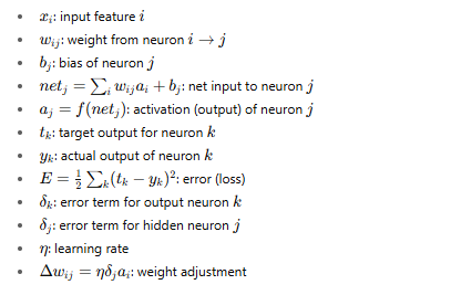
- x₁: Number of articles read in the past week
- x₂: Time spent on the site (in minutes) in the past month
- y: Subscription (1 = Yes, 0 = No)
| Visitor | x₁ (Articles Read) | x₂ (Time in Minutes) | y (Subscribed) |
|---|---|---|---|
| 1 | 6 | 180 | 1 |
| 2 | 3 | 60 | 0 |
| 3 | 8 | 240 | 1 |
| 4 | 2 | 30 | 0 |
| 5 | 5 | 120 | 1 |
🔧 Trained Logistic Regression Model:
- Intercept (b₀) = -2.5
- Coefficient for x₁ (b₁) = 0.4
- Coefficient for x₂ (b₂) = 0.01
🔍 Your Task:
Predict the subscription probability for a new visitor who:
- Read 4 articles (x₁ = 4)
- Spent 100 minutes (x₂ = 100)
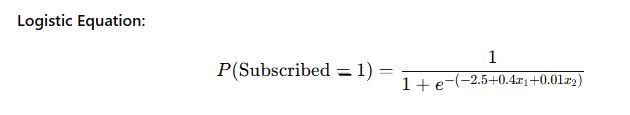
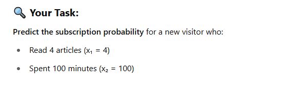
✅ Result:
The predicted subscription propensity is 52.5%.
Clustering
Clustering is a fundamental technique in the field of data analysis and machine learning that involves grouping a set of objects or data points into clusters, or subsets, such that objects within the same cluster are more similar to each other than to those in other clusters. The goal of clustering is to discover inherent structures or patterns in the data without any prior knowledge of class labels or predefined categories. It is an unsupervised learning method, meaning that the algorithm does not rely on labeled data but instead identifies relationships and similarities based on the input features.
Clustering plays a crucial role in many real-world applications, including market segmentation, image recognition, anomaly detection, and social network analysis. For example, businesses can use clustering to identify distinct customer segments, allowing them to tailor marketing strategies more effectively. In image recognition, clustering can help group similar images together based on visual features. Similarly, in social networks, clustering algorithms can identify communities of users with similar interests.
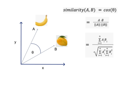
The process of clustering typically starts with the selection of a suitable similarity or distance measure, such as Euclidean distance, Manhattan distance, or cosine similarity, to quantify the closeness between data points. The choice of distance metric depends on the nature of the data and the problem at hand. Once a similarity measure is chosen, various clustering algorithms can be applied to partition the data into clusters. These algorithms vary in their approach and assumptions, but all share the common goal of grouping similar data points.
Several well-known clustering algorithms exist, each with its strengths and weaknesses. K-means is one of the most popular and widely used clustering algorithms. It works by partitioning the data into K clusters, where K is a user-defined parameter, and iteratively refines the cluster centroids until convergence. K-means is efficient and scalable, making it suitable for large datasets, but it has limitations, such as its sensitivity to the initial choice of cluster centroids and its assumption that clusters are spherical in-shape. Another well-known algorithm is hierarchical clustering, which builds a tree-like structure of nested clusters. Hierarchical clustering can be agglomerative, where clusters are progressively merged, or divisive, where clusters are split iteratively. This method does not require the number of clusters to be predefined and can provide a more intuitive understanding of the data’s structure. However, hierarchical clustering can be computationally expensive, especially for large datasets.
Density-based clustering methods, such as DBSCAN (Density-Based Spatial Clustering of Applications with Noise), are designed to find clusters of arbitrary shape and are particularly effective for datasets with noise and outliers. DBSCAN does not require the number of clusters to be specified in advance and instead relies on the density of points in a region to form clusters. This makes it suitable for scenarios where the number of clusters is not known beforehand or when clusters are not well-separated.
Clustering is an essential tool for exploratory data analysis, providing valuable insights into the inherent structure of data. By grouping similar objects together, it can reveal patterns that may not be immediately apparent, helping researchers, analysts, and practitioners make more informed decisions. However, clustering is not without its challenges, such as choosing the appropriate algorithm, determining the optimal number of clusters, and interpreting the results. Despite these challenges, clustering remains an invaluable technique in data-driven fields.
Clustering is an essential technique in data analysis and machine learning, which groups data points or objects into distinct clusters based on similarity. This unsupervised learning method enables the discovery of hidden patterns or structures in the data without the need for labeled examples. The goal is to identify natural groupings within the dataset so that items within the same group share certain characteristics while being dissimilar to items in other groups. Let’s explore clustering with detailed examples across various domains.
1. Market Segmentation in Business
A practical example of clustering can be found in market segmentation. Imagine a retail company that wants to identify different groups of customers based on their purchasing behaviors. The company gathers data on customer demographics, buying history, and preferences.
Process:
- Data points: Each customer is represented by a vector of features (age, income, frequency of purchase, product preferences, etc.).
- Clustering algorithm: K-means or DBSCAN could be used to group customers based on their purchasing patterns.
- Outcome: The algorithm might reveal distinct groups of customers, such as:
- Group 1: Young professionals who frequently purchase technology and gadgets.
- Group 2: Middle-aged parents who buy household items and children’s products.
- Group 3: Retired individuals who tend to buy health-related products.
Benefit: This segmentation allows the business to target each group with tailored marketing strategies, such as promotions on tech gadgets for Group 1 or discounts on health-related items for Group 3. It helps optimize resources and improve customer satisfaction.
2. Image Recognition in Computer Vision
Clustering can be used to group similar images for classification or recognition tasks. Suppose a company wants to organize a large collection of photos, say from a social media platform, into categories such as “landscapes,” “portraits,” and “animals.”
Process:
- Data points: Each image is represented by a vector of features, such as color histograms, edge detection patterns, or deep learning features extracted from pre-trained neural networks.
- Clustering algorithm: K-means or hierarchical clustering could be used to group similar images based on these features.
- Outcome: The algorithm might categorize the images into:
- Cluster 1: Images of natural landscapes, such as mountains, forests, and beaches.
- Cluster 2: Portraits or selfies with faces.
- Cluster 3: Animals, including cats, dogs, and wildlife.
Benefit: Clustering simplifies organizing vast image datasets, making it easier for users to browse and search through photos. It could also support automated tagging or categorization of new images as they are uploaded.
3. Anomaly Detection in Fraud Detection
Clustering can be helpful in identifying unusual patterns or outliers within data, which is particularly useful in fraud detection. For instance, a bank may want to detect fraudulent transactions based on customer behavior.
Process:
- Data points: Each transaction is represented by features such as transaction amount, frequency, location, and time.
- Clustering algorithm: DBSCAN (Density-Based Spatial Clustering of Applications with Noise) is effective in this case, as it can find clusters of normal transactions while identifying transactions that do not belong to any cluster (outliers).
- Outcome: Most transactions fall into clusters representing regular customer behavior. However, some transactions, such as a large withdrawal from a foreign country, will not belong to any cluster, signaling potentially fraudulent activity.
Benefit: By automatically detecting transactions that deviate from normal patterns, banks can flag suspicious activities for further investigation, preventing fraud and ensuring security.
4. Social Network Analysis
In social networks, clustering algorithms can help detect communities of users who share common interests or social connections. For example, an online platform like Twitter might want to identify groups of users with similar interests to recommend relevant content.
Process:
- Data points: Each user is represented by a set of features such as the number of followers, topics of posts, and interactions with others.
- Clustering algorithm: Spectral clustering or community detection algorithms (like the Louvain method) can be applied to find communities.
- Outcome: The algorithm might identify several communities of users, such as:
- Community 1: Sports enthusiasts discussing football and basketball.
- Community 2: Food lovers sharing recipes and restaurant reviews.
- Community 3: Environmental activists focusing on climate change and sustainability.
Benefit: This clustering helps the platform recommend relevant posts or users to follow, improving user engagement and experience.
5. Genetic Data Analysis in Biology
Clustering can be used in biology to group genes or species with similar genetic traits. For example, researchers might want to identify clusters of genes that are involved in the same biological pathways.
Process:
- Data points: Each gene is represented by a vector of expression levels across various conditions or tissues.
- Clustering algorithm: Hierarchical clustering or K-means could be used to identify genes with similar expression patterns.
- Outcome: The algorithm might reveal groups of genes, such as:
- Cluster 1: Genes highly expressed during the immune response.
- Cluster 2: Genes associated with cell growth and division.
- Cluster 3: Genes that are more active during stress conditions.
Benefit: Clustering genes based on their expression patterns can help researchers understand biological processes and identify potential targets for drug development.
Clustering is a versatile and powerful tool used across many fields for uncovering hidden patterns, categorizing data, and making sense of complex datasets. Whether for market segmentation, image recognition, fraud detection, social network analysis, or genetic research, clustering provides valuable insights that can drive decision-making and improve outcomes. Despite its challenges, such as determining the right number of clusters and handling noisy data, clustering remains one of the most important methods in data science and machine learning.
k-means clustering
K-Means clustering is one of the most popular and widely used unsupervised machine learning algorithms, designed to partition a set of data points into a predefined number of clusters, K. The primary goal of K-Means is to group data points in such a way that data points within the same cluster are more similar to each other than to those in other clusters. This is achieved through a process of iterative refinement, where the algorithm repeatedly assigns data points to clusters and then updates the cluster centroids until the clustering stabilizes.
How K-Means Clustering Works
K-Means works in the following steps:
- Initialization: The algorithm begins by selecting K initial centroids (one for each cluster). These centroids can either be chosen randomly from the data points or selected using more sophisticated methods like the K-Means++ algorithm, which aims to spread out the initial centroids to improve the clustering process.
- Assignment Step: Each data point is assigned to the nearest centroid. The “nearest” centroid is determined based on a chosen distance metric, typically Euclidean distance, which measures the straight-line distance between a data point and the centroid.
- Update Step: After all data points have been assigned to clusters, the centroids are recalculated. The new centroid of each cluster is the mean (average) of all the points assigned to that cluster. This means that the new centroid is the point that minimizes the sum of squared distances to all points within the cluster.
- Repeat: The assignment and update steps are repeated iteratively. In each iteration, data points may be reassigned to different clusters, and centroids are updated accordingly. This continues until the assignments no longer change, or until a predefined number of iterations is reached, signaling convergence.
Example of K-Means Clustering
Consider a simple example where we have a dataset of customer purchasing behavior, with two features: income and spending score. We want to group the customers into K=3 clusters based on these features.
- Initialization: Suppose K=3, so we randomly select three initial centroids from the data points.
- Assignment: Each customer is assigned to the closest centroid based on their income and spending score.
- Update: After assigning customers to the clusters, we calculate the mean income and spending score for each group and update the centroids.
- Repeat: The steps are repeated until the customer assignments no longer change, and the final clusters represent groups of customers with similar spending patterns.
Key Characteristics of K-Means
- Efficiency: K-Means is computationally efficient and scales well with large datasets. Its time complexity is typically O(n * K * I), where n is the number of data points, K is the number of clusters, and I is the number of iterations. This makes it faster than many other clustering algorithms, especially when working with large datasets.
- Convergence: K-Means converges to a local optimum solution, meaning that it will find a solution that is optimal in terms of minimizing the sum of squared distances within each cluster, but it is not guaranteed to find the global optimum. The outcome can depend on the initial selection of centroids.
- Assumptions: K-Means assumes that clusters are spherical and of roughly equal size. This means that it may not perform well when clusters are of different shapes or densities.
- Sensitivity to Initialization: The performance of K-Means can be heavily influenced by the initial selection of centroids. Poor initialization can lead to suboptimal clustering. This is why methods like K-Means++ were introduced to improve the selection of initial centroids and reduce the chance of poor results.
Strengths and Limitations of K-Means
Strengths:
- Simple and easy to understand.
- Fast and scalable, making it suitable for large datasets.
- Versatile and can be used in a variety of domains, from market segmentation to image compression.
Limitations:
- The number of clusters (K) must be specified in advance, which can be challenging without prior knowledge of the data.
- It can be sensitive to outliers, which may distort the final clusters.
- The assumption of spherical clusters means K-Means may not perform well on datasets with non-spherical or highly imbalanced clusters.
- It may converge to a local minimum, not necessarily the global optimal solution.
Applications of K-Means
K-Means is used in a wide variety of real-world applications, including:
- Customer Segmentation: Grouping customers based on purchasing behavior to tailor marketing strategies.
- Image Compression: Reducing the size of image files by clustering similar pixel values and representing them with the average value.
- Document Clustering: Grouping documents with similar content in information retrieval systems.
- Anomaly Detection: Identifying unusual patterns by clustering normal data points and flagging outliers.
Conclusion
K-Means clustering is a powerful and efficient algorithm for grouping data points into clusters based on similarity. Despite its simplicity, it is widely used in various fields due to its scalability, ease of use, and effectiveness in uncovering patterns in large datasets. However, it is important to consider its limitations, such as sensitivity to initialization and the need for a predefined number of clusters. Despite these challenges, K-Means remains one of the most popular clustering algorithms in data analysis and machine learning.
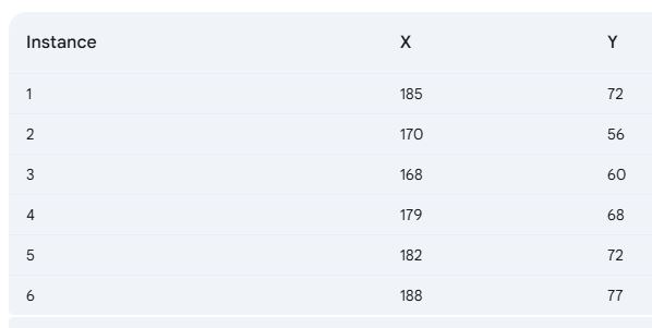
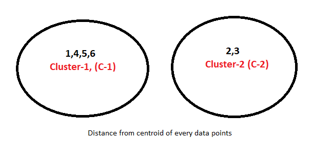
Implement the K-Means algorithm with K = 2 on the data points (185, 72), (170, 56), (168, 60), (179, 68), (182, 72), and (188, 77) for two iterations, and display the resulting clusters. Initially, select the first two data points as the initial centroids.
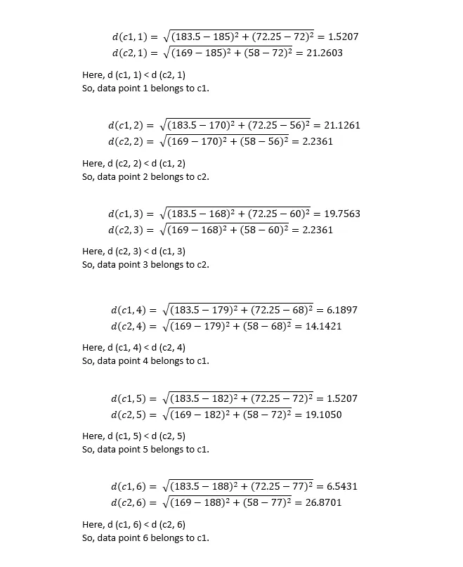
In the initial step, we determine the similarity between data points using the Euclidean distance metric.
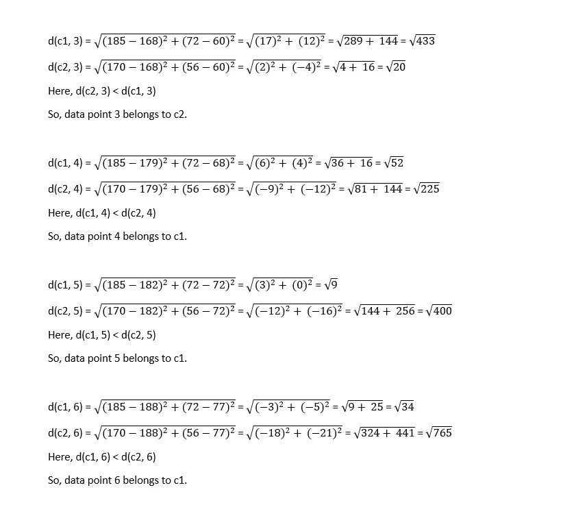
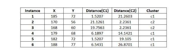
In tabular-form it can be represented as,

The result after first iteration.
In the second iteration, calculating centroids again,

Calculating distances again,
In tabular form,
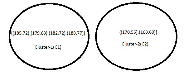
As two iterations have already been completed as required by the problem, the numerical process concludes here. Since the clustering remains unchanged after the second iteration, the process will be terminated, even if the question does not explicitly state to do so.
#Python code for K means clustering
import pandas as pd
from sklearn.cluster import KMeans

# Sample data from the image
data = {'Instance': [1, 2, 3, 4, 5, 6],
        'X': [185, 170, 168, 179, 182, 188],
        'Y': [72, 56, 60, 68, 72, 77]}

df = pd.DataFrame(data)

# Select features for clustering
X = df[['X', 'Y']]

# Choose the number of clusters (K)
num_clusters = 2  # You can adjust this value

# Create a KMeans object
kmeans = KMeans(n_clusters=num_clusters, random_state=42)

# Fit the model to the data
kmeans.fit(X)

# Get cluster labels for each data point
labels = kmeans.labels_

# Adjust cluster labels to start from 1
adjusted_labels = labels + 1

# Add adjusted cluster labels to the DataFrame
df['Cluster'] = adjusted_labels

# Print the clustered data
print(df)

Output:
   Instance     X     Y  Cluster
0         1  185.0  72.0       1
1         2  170.0  56.0       2
2         3  168.0  60.0       2
3         4  179.0  68.0       1
4         5  182.0  72.0       1
5         6  188.0  77.0       1
Collaborative Filtering
Introduction to Collaborative Filtering and Recommendation Systems
Recommendation systems are algorithms used to suggest items to users based on various criteria, such as past behavior, preferences, and the behavior of similar users. Collaborative filtering is one of the most widely used techniques for building recommendation systems. It works by making recommendations based on the preferences or ratings of other users who are similar to the target user.
There are generally two types of recommendation systems:
- Collaborative Filtering: Uses the past behaviors and ratings of users to recommend items.
- User-based Collaborative Filtering: Recommends items based on similarities between users.
- Item-based Collaborative Filtering: Recommends items that are similar to items the user has liked before.
- Content-Based Filtering: Recommends items based on the attributes of the items and the user’s past interactions with those attributes.
- Hybrid Models: Combines both collaborative and content-based approaches to provide better recommendations.
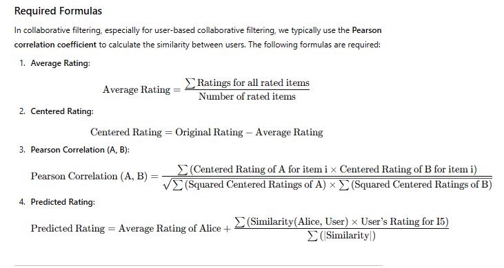
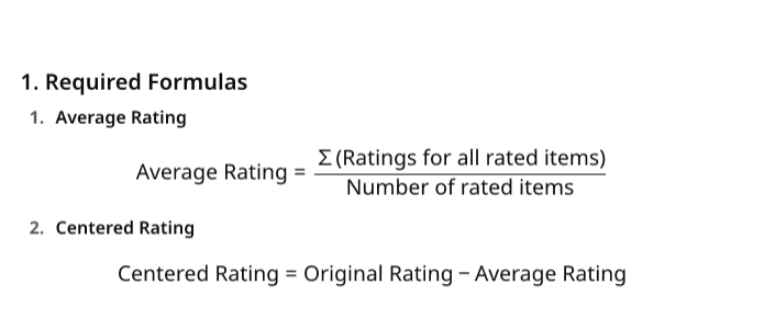
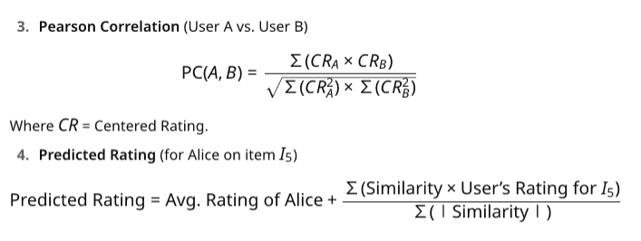
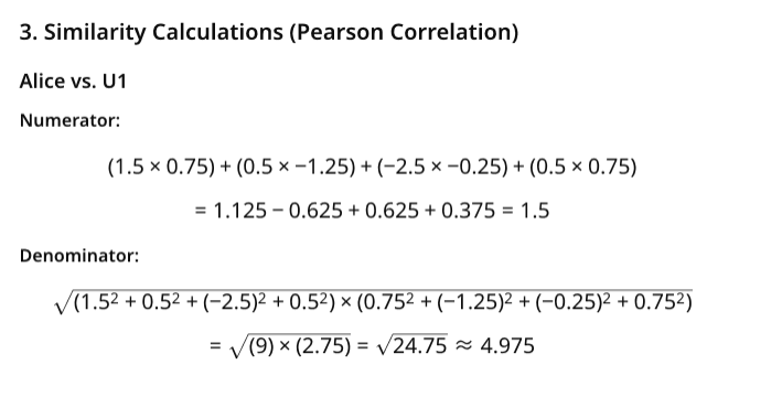
Required Formulas
In collaborative filtering, especially for user-based collaborative filtering, we typically use the Pearson correlation coefficient to calculate the similarity between users. The following formulas are required:
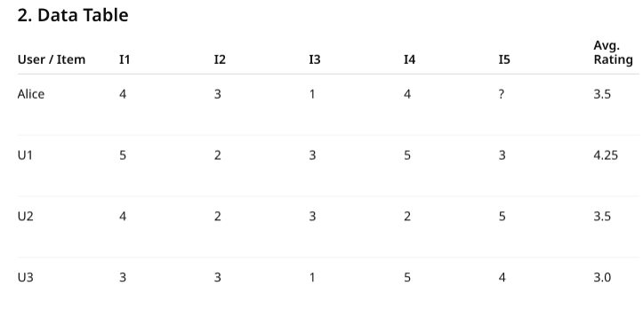
1. Data Preparation
Original Rating Matrix:
| User | Inshorts (I1) | HT (I2) | NYT (I3) | TOI (I4) | BBC (I5) |
|---|---|---|---|---|---|
| Alice | 5 | 4 | 1 | 4 | ? |
| U1 | 3 | 1 | 2 | 3 | 3 |
| U2 | 4 | 3 | 4 | 3 | 5 |
| U3 | 3 | 3 | 1 | 5 | 4 |
2. Calculate Average Ratings for Each User
Formula:
Average Rating = (Sum of Ratings for all rated items) / (Number of rated items)
| User | Inshorts (I1) | HT (I2) | NYT (I3) | TOI (I4) | Average Rating |
|---|---|---|---|---|---|
| Alice | 5 | 4 | 1 | 4 | 3.5 |
| U1 | 3 | 1 | 2 | 3 | 2.25 |
| U2 | 4 | 3 | 4 | 3 | 3.5 |
| U3 | 3 | 3 | 1 | 5 | 3 |
Average Ratings:
- Alice: (5 + 4 + 1 + 4) / 4 = 3.5
- U1: (3 + 1 + 2 + 3) / 4 = 2.25
- U2: (4 + 3 + 4 + 3) / 4 = 3.5
- U3: (3 + 3 + 1 + 5) / 4 = 3
3. Center the Ratings (Subtract Average Rating from Each Rating)
Formula:
Centered Rating = Original Rating – Average Rating
| User | Inshorts (I1) | HT (I2) | NYT (I3) | TOI (I4) | BBC (I5) |
|---|---|---|---|---|---|
| Alice | 1.5 | 0.5 | -2.5 | 0.5 | ? |
| U1 | 0.75 | -1.25 | -0.25 | 0.75 | ? |
| U2 | 0.5 | -0.5 | 0.5 | -0.5 | ? |
| U3 | 0 | 0 | -2 | 2 | ? |
Centered Ratings Calculation:
- Alice:
- Inshorts (I1) = 5 – 3.5 = 1.5
- HT (I2) = 4 – 3.5 = 0.5
- NYT (I3) = 1 – 3.5 = -2.5
- TOI (I4) = 4 – 3.5 = 0.5
- U1:
- Inshorts (I1) = 3 – 2.25 = 0.75
- HT (I2) = 1 – 2.25 = -1.25
- NYT (I3) = 2 – 2.25 = -0.25
- TOI (I4) = 3 – 2.25 = 0.75
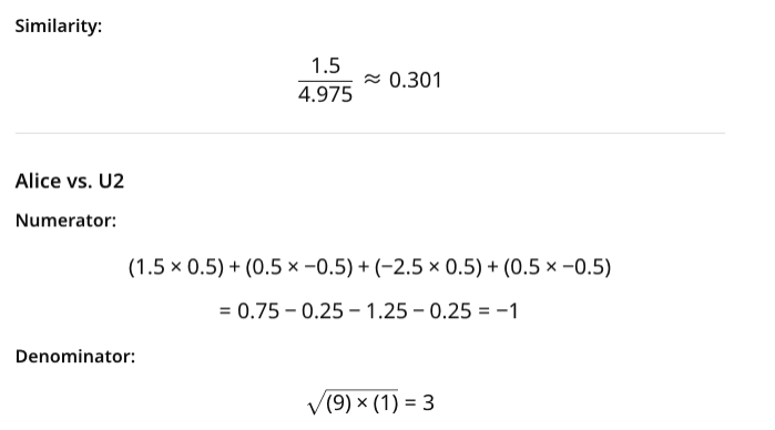
- U2:
- Inshorts (I1) = 4 – 3.5 = 0.5
- HT (I2) = 3 – 3.5 = -0.5
- NYT (I3) = 4 – 3.5 = 0.5
- TOI (I4) = 3 – 3.5 = -0.5
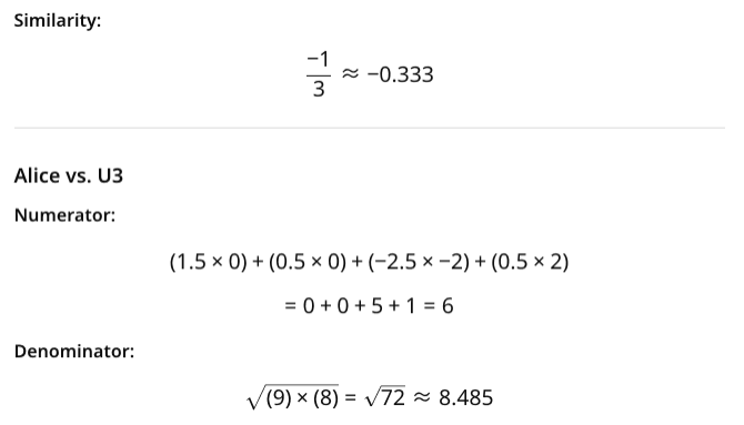
- U3:
- Inshorts (I1) = 3 – 3 = 0
- HT (I2) = 3 – 3 = 0
- NYT (I3) = 1 – 3 = -2
- TOI (I4) = 5 – 3 = 2


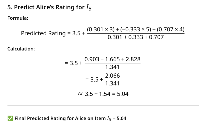
Alice’s predicted rating for BBC News (I5) is approximately 5.04.
This prediction is based on the weighted average of Alice’s similarities with other users and their respective ratings for BBC News.
Here is the Python code to solve the collaborative filtering problem you provided. This code will:
- Calculate the average ratings for each user.
- Center the ratings.
- Calculate the Pearson similarity between users.
- Predict Alice’s rating for BBC News (I5).
import numpy as np

# Original Rating Matrix
ratings = {
    'Alice': [5, 4, 1, 4, None],
    'U1': [3, 1, 2, 3, 3],
    'U2': [4, 3, 4, 3, 5],
    'U3': [3, 3, 1, 5, 4]
}

# Calculate Average Rating for each user
def calculate_average_rating(ratings):
    average_ratings = {}
    for user, user_ratings in ratings.items():
        # Calculate average of non-None ratings
        valid_ratings = [rating for rating in user_ratings if rating is not None]
        average_ratings[user] = sum(valid_ratings) / len(valid_ratings)
    return average_ratings

# Center the ratings by subtracting the average rating
def center_ratings(ratings, average_ratings):
    centered_ratings = {}
    for user, user_ratings in ratings.items():
        centered_ratings[user] = [rating - average_ratings[user] if rating is not None else None for rating in user_ratings]
    return centered_ratings

# Calculate Pearson similarity between two users
def pearson_similarity(user1, user2, centered_ratings):
    common_ratings = []
    for i in range(len(user1)):
        if centered_ratings[user1][i] is not None and centered_ratings[user2][i] is not None:
            common_ratings.append(i)

    if not common_ratings:
        return 0

    numerator = sum(centered_ratings[user1][i] * centered_ratings[user2][i] for i in common_ratings)
    denominator = np.sqrt(sum(centered_ratings[user1][i] ** 2 for i in common_ratings)) * np.sqrt(sum(centered_ratings[user2][i] ** 2 for i in common_ratings))

    return numerator / denominator if denominator != 0 else 0

# Predict Alice's rating for BBC News (I5)
def predict_rating(user, target_item, ratings, centered_ratings, average_ratings):
    similarities = []
    weighted_ratings = []

    for other_user in ratings:
        if other_user != user and ratings[other_user][target_item] is not None:
            similarity = pearson_similarity(user, other_user, centered_ratings)
            similarities.append((other_user, similarity))
            weighted_ratings.append(similarity * ratings[other_user][target_item])

    if not similarities:
        return average_ratings[user]

    total_similarity = sum(abs(similarity) for _, similarity in similarities)
    predicted_rating = average_ratings[user] + sum(weighted_ratings) / total_similarity if total_similarity != 0 else average_ratings[user]

    return predicted_rating

# Main program to calculate everything
average_ratings = calculate_average_rating(ratings)
centered_ratings = center_ratings(ratings, average_ratings)

# Predict Alice's rating for BBC News (I5), which is index 4
predicted_rating = predict_rating('Alice', 4, ratings, centered_ratings, average_ratings)

# Output
print(f"Alice's predicted rating for BBC News (I5): {predicted_rating:.2f}")

Output:
Alice's predicted rating for BBC News (I5): 5.04

//Explanation of Code:
calculate_average_rating: This function calculates the average rating for each user by summing all the ratings and dividing by the number of ratings (excluding None values).

center_ratings: This function centers the ratings for each user by subtracting the user's average rating from each of their ratings.

pearson_similarity: This function calculates the Pearson similarity between two users based on their centered ratings.

predict_rating: This function predicts the rating for a given user and item (in this case, Alice's rating for BBC News, I5). It uses Pearson similarity to compute a weighted average of ratings from similar users.
Collaborative Filtering using Jaccard Similarrity
Collaborative Filtering using Cosine Similarrity
Linear Regression
Multiple Linear Regression
Logistic Regression
Regression tree
A regression tree is a type of decision tree adapted for regression problems, where the target variable is continuous rather than categorical. While traditional decision trees—like ID3, C4.5, and CART—are primarily designed for classification tasks, regression trees use similar principles but apply different metrics to split the data. Instead of focusing on metrics like information gain, gain ratio, or the Gini index (used for classification), regression trees typically use metrics related to minimizing error, such as variance reduction or mean squared error (MSE).
The most common algorithm for building regression trees is the CART (Classification and Regression Trees) algorithm. While CART works for classification tasks by using the Gini index, for regression problems, CART adapts by using the variance of the target variable as the criterion for splitting nodes.
Step-by-Step Guide for Regression Trees with CART:
Let’s walk through a simple example using the same dataset used for classification in a prior experiment (golf playing decision). However, in this case, the target variable represents the number of golf players, which is a continuous numerical value rather than a categorical one (like true/false in the original experiment).
1. Data Understanding
In the previous classification version of this dataset, the target column represented the decision to play golf (True/False). Here, the target column represents the number of golf players, which is a real number. The features might be the same (e.g., weather conditions, time of day), but the key difference is that the target is continuous rather than categorical.
2. Handling Continuous Target Variable
Since the target is now a continuous variable, we cannot use traditional classification metrics like counting occurrences of “True” and “False.” Instead, we use the variance of the target variable as a way to decide how to split the data. The objective is to reduce the variance within each subset after a split.
3. Splitting the Data (Using Variance)
- For each potential split, we calculate the variance (or standard deviation) of the target variable in the two child nodes.
- The goal is to choose the split that results in the largest reduction in variance. The split with the least variance in each subset will indicate the most “homogeneous” groups with respect to the target variable.
4. Recursive Process
- The tree-building process proceeds recursively. After finding the best split based on variance reduction, the dataset is divided into two subsets. The same process is then applied to each of these subsets until the stopping criteria are met (e.g., a maximum tree depth or a minimum number of data points in a leaf node).
5. Prediction with Regression Tree
- Once the tree is built, each leaf node will contain the predicted value for the target variable. For regression trees, the value predicted by a leaf node is typically the mean of the target variable for the instances in that leaf.
- New instances are passed down the tree, and the prediction is made by reaching a leaf and taking the average of the target values in that leaf.
6. Pruning the Tree
- Just like classification trees, regression trees can be prone to overfitting. A tree that grows too deep may model noise in the data, leading to poor generalization. To counter this, pruning can be applied, which involves cutting back some branches of the tree to improve performance on unseen data.
Example with the Golf Dataset:
In the golf dataset, where we have the number of golf players as the target variable, we might use weather conditions or time of day as the features. Since the target variable is a continuous value (e.g., the number of players), the algorithm would calculate the variance of the number of players within different subsets of the data based on these features. The tree would split the data based on the feature that most reduces this variance at each step.
For instance, if the weather condition (e.g., sunny or rainy) significantly reduces the variance of the number of players, this would be chosen as a splitting criterion. The process continues recursively until the tree reaches a satisfactory depth or further splits no longer reduce variance significantly.
Regression trees serve as powerful tools for handling continuous target variables, and the CART algorithm adapts this idea by focusing on minimizing variance within subsets rather than classifying instances into discrete classes. This enables decision trees to make classifications and predict continuous outcomes effectively.
Non-Linear Polynomial Regression
Detail Calculations of the above steps 4,5 & 6
What is Partial Least Squares (PLS) Regression?
PLS Regression is a statistical method that combines features of principal component analysis (PCA) and multiple regression.
Its goal is to find latent components (linear combinations of predictors) that explain as much as possible of the covariance between predictors XXX and response YYY.
PLS is especially useful when:
- Predictors are highly correlated (multicollinearity problem).
- Number of predictors > number of observations (high-dimensional data).
Classification-Non Linear
Bayesian classification
Bayesian classification(Real Values)
Neural Network-Part A
Neural Network-Part B
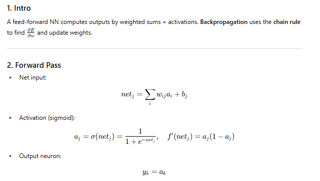
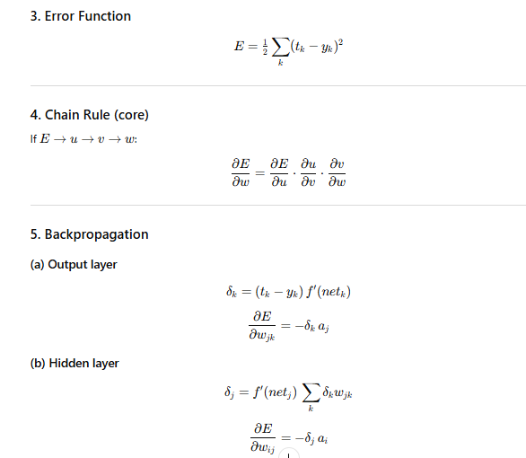
Backpropagation NN
Backpropagation is a learning algorithm for neural networks that works in two steps: first, the error between the predicted output and the target is calculated; then, using the chain rule of calculus, this error is propagated backward through the network to compute gradients for each weight. These gradients are then used to update the weights and improve the model’s accuracy.


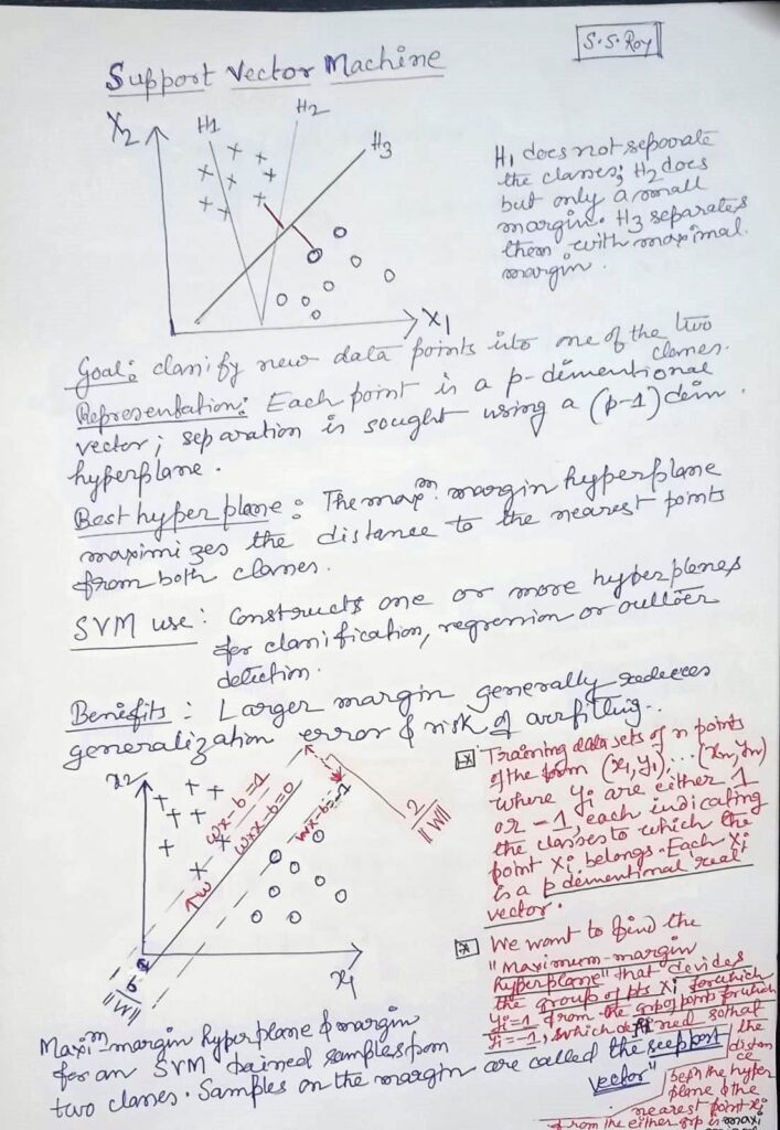
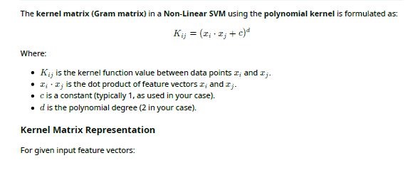
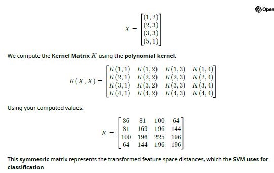
Support Vector Machine(SVM)
SVM-PART-B(Simplified explanation)


SVM-Non Linear
Decision Tree: C4.5
Model Evaluation Metrics: Classification
Class Imbalance
Understanding Class Imbalance: Concepts and Challenges
Class imbalance is a pervasive issue in many real-world machine learning problems, especially in domains like fraud detection, medical diagnosis, anomaly detection, and rare event prediction, where the number of examples in one class significantly outweighs the others. In a typical binary classification scenario, a balanced dataset might contain roughly equal numbers of positive and negative samples, but with class imbalance, one class (majority) dominates the other (minority), leading to a skewed distribution. For instance, in a cancer detection dataset, healthy patients may represent 98% of the data, while only 2% represent the cancer-positive cases. This disparity poses challenges for standard classification algorithms, which tend to be biased towards the majority class, often resulting in high overall accuracy but poor recall for the minority class. Accuracy becomes a misleading metric in such cases, as a model predicting only the majority class can still achieve high accuracy while completely ignoring the minority class. Therefore, metrics like precision, recall, F1-score, area under the ROC curve (AUC-ROC), and confusion matrix analysis are preferred for evaluating performance in imbalanced settings. Moreover, class imbalance affects model learning by minimizing the influence of rare class patterns, leading to underfitting for minority class features. As a result, without proper handling, imbalanced datasets can result in models that are ill-equipped to make meaningful predictions about the minority class, which is often the most important class in critical applications.
To address class imbalance, several techniques can be applied during data preprocessing, algorithm design, and evaluation. Resampling methods are widely used and include undersampling the majority class, oversampling the minority class, or employing synthetic data generation techniques like SMOTE (Synthetic Minority Oversampling Technique), which creates new minority class samples by interpolating between existing ones. While undersampling can lead to loss of potentially useful data, oversampling may cause overfitting due to repetition. Algorithm-level strategies, such as cost-sensitive learning, introduce penalty terms for misclassifying the minority class, thus guiding the model to pay more attention to it. Ensemble methods like Random Forest, Boosting (especially AdaBoost or XGBoost with appropriate parameter tuning), and hybrid techniques combining sampling with ensembles have shown effectiveness. Recent advances also include generative models and deep learning architectures that incorporate class reweighting or use focal loss to concentrate on hard-to-classify minority instances. Additionally, techniques like threshold moving, data augmentation, and transfer learning are gaining popularity in addressing imbalance. It is crucial to select appropriate evaluation metrics and visualize learning performance through tools like precision-recall curves or class-specific confusion matrices to ensure that the model generalizes well across all classes. Ultimately, handling class imbalance is not a one-size-fits-all solution—it requires a thoughtful combination of strategies, tailored experimentation, and iterative refinement to develop robust, fair, and reliable machine learning models that perform equitably across all classes, especially the underrepresented ones.