K-MEANS CLUSTERING
K-Means clustering is a powerful and efficient algorithm for grouping data points into clusters based on similarity. Despite its simplicity, it is widely used in various fields due to its scalability, ease of use, and effectiveness in uncovering patterns in large datasets. However, it is important to consider its limitations, such as sensitivity to initialization and the need for a predefined number of clusters. Despite these challenges, K-Means remains one of the most popular clustering algorithms in data analysis and machine learning.
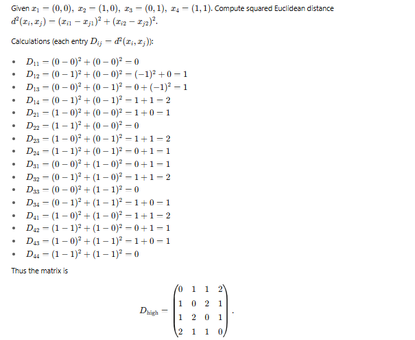
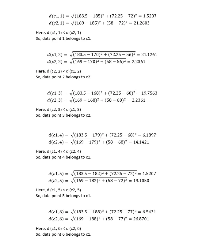
Implement the K-Means algorithm with K = 2 on the data points (185, 72), (170, 56), (168, 60), (179, 68), (182, 72), and (188, 77) for two iterations, and display the resulting clusters. Initially, select the first two data points as the initial centroids.

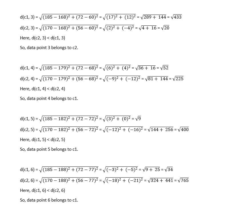
In the initial step, we determine the similarity between data points using the Euclidean distance metric.
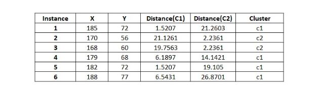
In tabular-form it can be represented as,
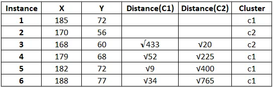
The result after first iteration.

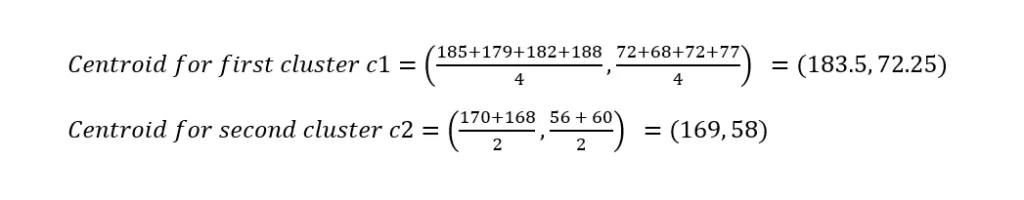
In the second iteration, calculating centroids again,
Calculating distances again,
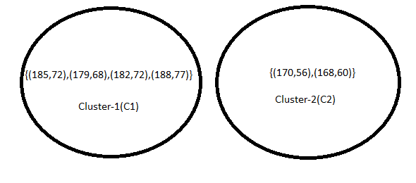
As two iterations have already been completed as required by the problem, the numerical process concludes here. Since the clustering remains unchanged after the second iteration, the process will be terminated, even if the question does not explicitly state to do so.
Read more: Unsupervised learningK-MODES CLUSTERING
Hierarchical Clustering
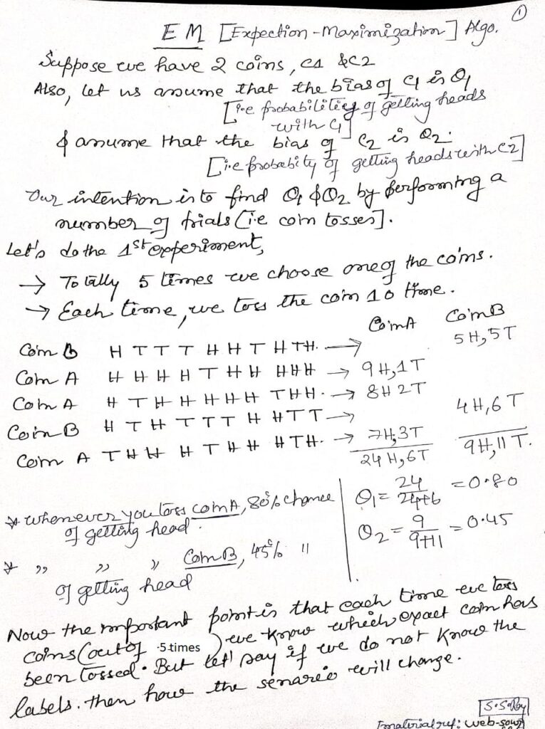
Expectation-Maximization (EM) Algorithm
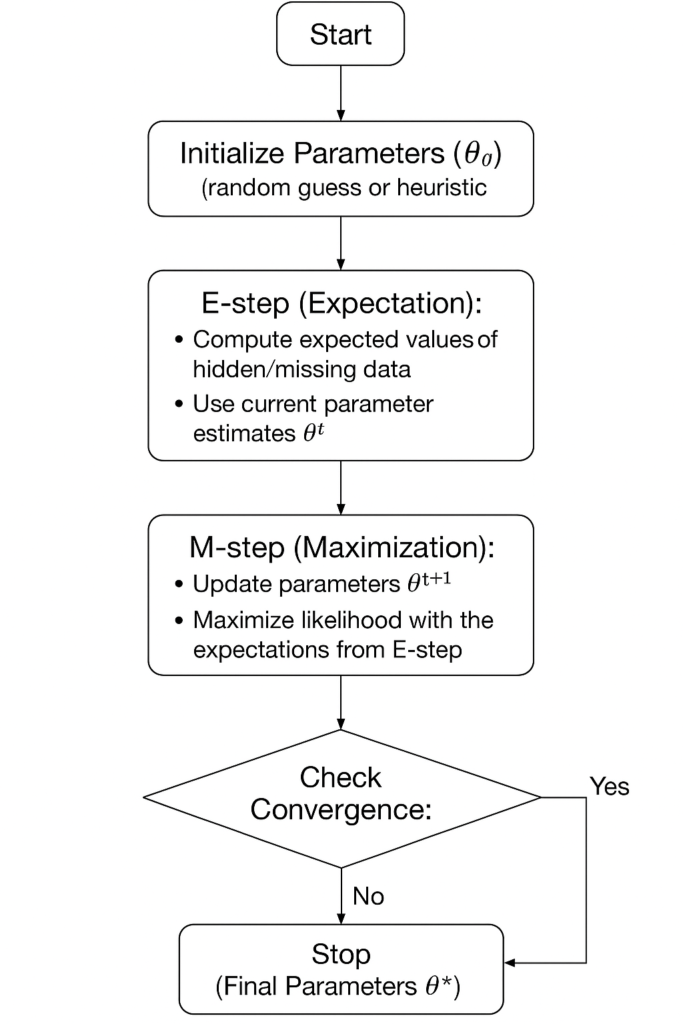
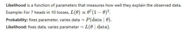
The Expectation-Maximization (EM) algorithm is a powerful iterative method to estimate parameters of probabilistic models when data is incomplete, uncertain, or involves hidden variables.
- Idea: Direct maximization of likelihood is hard due to missing/hidden data. EM solves this by alternating between two intuitive steps:
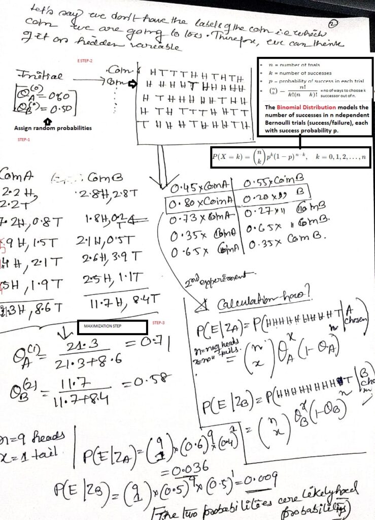
- E-step (Expectation): Compute the expected value of hidden variables using current parameters.
- M-step (Maximization): Update parameters by maximizing the likelihood with these expectations.
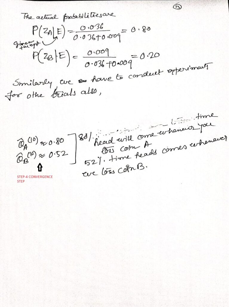
This repeat–refine process guarantees non-decreasing likelihood and converges to a local optimum. EM underlies key methods like Gaussian Mixture Models, Hidden Markov Models, and clustering with incomplete data, making it a cornerstone of statistical learning.
Other applications : Image Processing: Segmentation, denoising;Missing Data Problems: Robust parameter estimation;Anomaly Detection: Fraud, outliers.,Medical & Bioinformatics: Gene expression, disease models;Recommender Systems: Latent factor models.
Mathematical Prerequisites:
MCQs on EM
- What is the main purpose of the EM algorithm?
A) Solve linear equations
B) Maximize likelihood with incomplete data
C) Minimize squared error
D) Perform gradient descent
Answer: B) Maximize likelihood with incomplete data - Which two main steps does EM consist of?
A) Encode and Decode
B) Expectation and Maximization
C) Sampling and Updating
D) Forward and Backward
Answer: B) Expectation and Maximization - EM is typically used when:
A) All data is observed
B) Data is incomplete or has latent variables
C) The dataset is small
D) The data is categorical only
Answer: B) Data is incomplete or has latent variables - The EM algorithm guarantees:
A) Convergence to global maximum likelihood
B) Convergence to a local maximum of likelihood
C) Exact posterior distributions
D) Linear convergence speed
Answer: B) Convergence to a local maximum of likelihood
- In the Gaussian Mixture Model (GMM), what does the E-step compute?
A) Update the means of clusters
B) Update the covariance matrices
C) Compute responsibilities (probabilities of points belonging to clusters)
D) Compute the gradient of the likelihood
Answer: C) Compute responsibilities (probabilities of points belonging to clusters) - Which of the following is a limitation of EM?
A) Requires derivative computations
B) Sensitive to initial parameter values
C) Can only handle two clusters
D) Works only with discrete data
Answer: B) Sensitive to initial parameter values - After how many iterations does EM converge?
A) Always in one iteration
B) Depends on the convergence criterion (e.g., change in likelihood)
C) Always after 10 iterations
D) EM never converges
Answer: B) Depends on the convergence criterion (e.g., change in likelihood) - Which of these is true about the log-likelihood in EM?
A) It decreases in each iteration
B) It increases or stays the same in each iteration
C) It oscillates randomly
D) It remains constant
Answer: B) It increases or stays the same in each iteration
- Consider EM applied to a mixture of two Gaussians with identical variances. If the initial means are very close, which problem can occur?
A) The algorithm will converge to the true global maximum
B) The algorithm may converge to a degenerate solution or local maximum
C) The E-step cannot be computed
D) The covariance will become negative
Answer: B) The algorithm may converge to a degenerate solution or local maximum - Which mathematical property of the EM algorithm ensures the likelihood never decreases?
A) Jensen’s inequality
B) Cauchy-Schwarz inequality
C) Bayes’ theorem
D) Law of Large Numbers
Answer: A) Jensen’s inequality
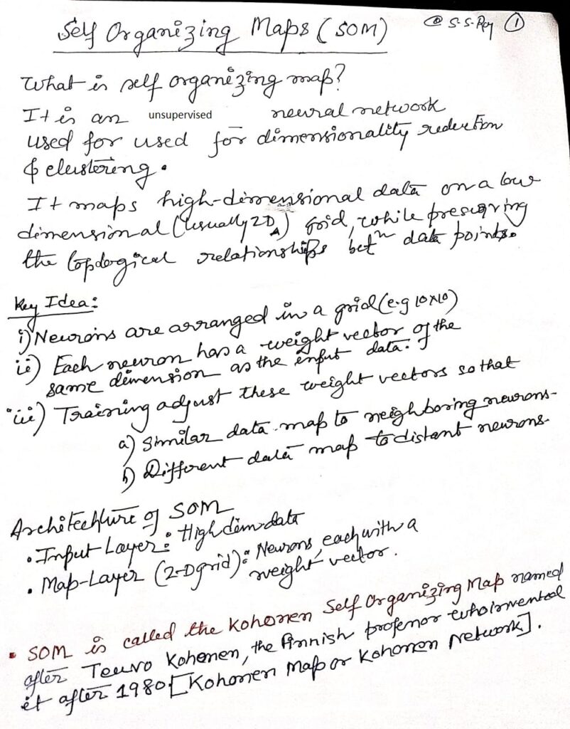
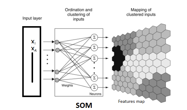
Self Organizing Maps(SOM)
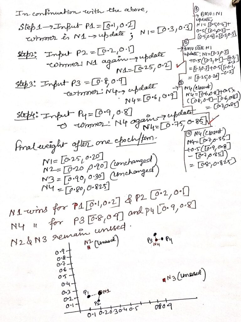
POINTS TO REMEMBER–>
- Unsupervised neural network using competitive, neighborhood-based weight adaptation.
- Preserves topological relationships: nearby neurons map nearby inputs.
- Dimensionality reduction alternative to PCA, nonlinear manifold preserving.
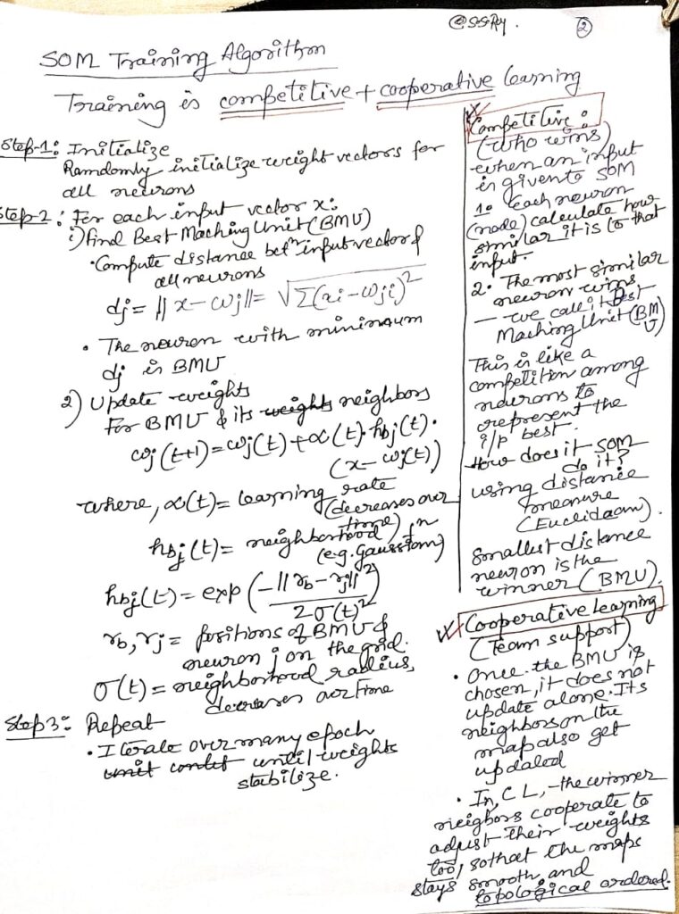
- Converges via decreasing learning rate and shrinking neighborhood radius.
- Applications: clustering, visualization, anomaly detection, feature extraction.
- SOM scales poorly; parallel GPU/mini-batch training mitigates complexity.
- Topology choice (hexagonal vs rectangular grid) impacts neighborhood smoothing.
- Initialization (PCA-based vs random) strongly influences convergence stability.
- Quantization error and topographic error are key SOM evaluation metrics.
- Used for high-dimensional clustering in genomics, NLP embeddings, finance.
PCA
PCA (Principal Component Analysis) is a statistical method used to reduce the number of variables (dimensions) in a large dataset while retaining most of the original data’s variation and information. It does this by converting the data into new, independent variables called principal components, which help simplify complex data, improve visualizations, boost machine learning model performance, and make datasets easier to analyze and interpret.
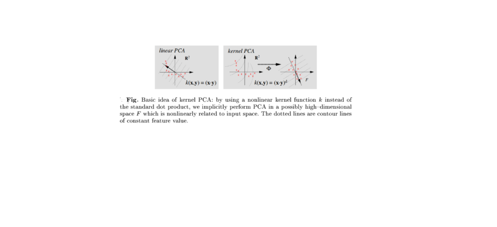
PCA-KERNEL
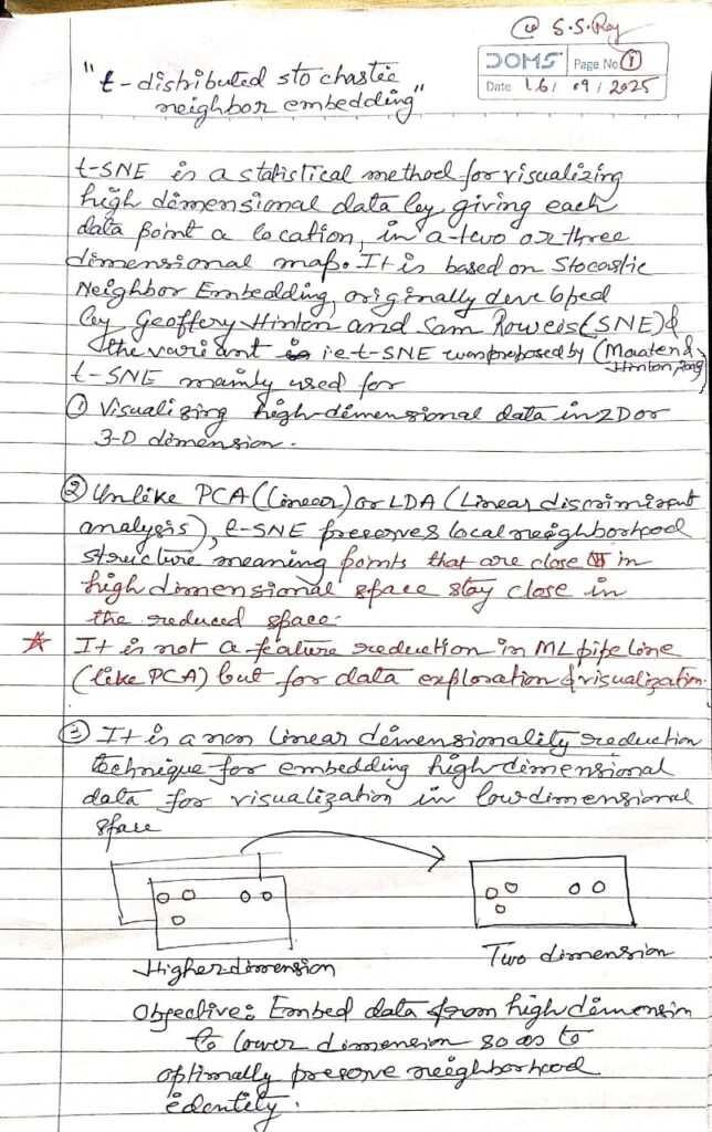
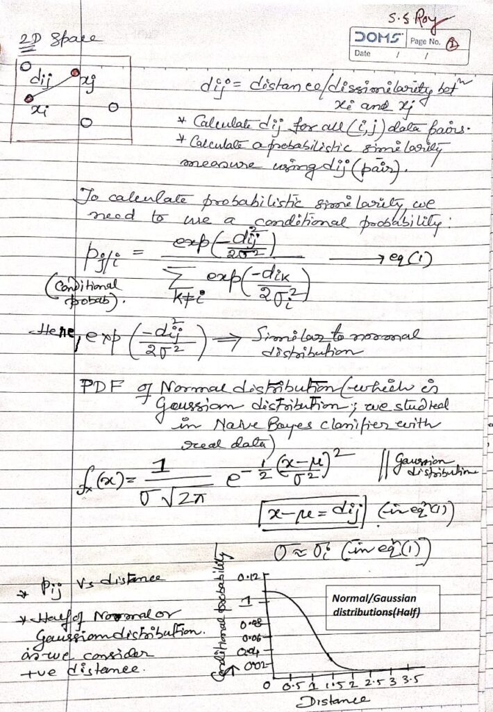
t-SNE (t-distributed Stochastic Neighbor Embedding)
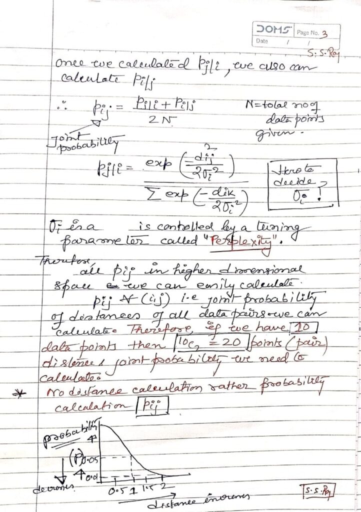
t-SNE (t-distributed Stochastic Neighbor Embedding), introduced by Laurens van der Maaten and Geoffrey Hinton (2008), is a non-linear dimensionality reduction technique, mainly used for visualizing high-dimensional data in 2D or 3D.
Important points->
How does perplexity influence structure?
→ Balances local detail vs. global cluster relationships.
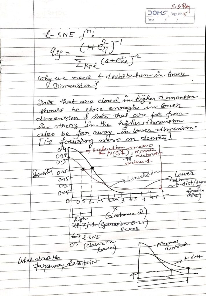
Why Student-t distribution instead of Gaussian?
→ Heavy tails prevent crowding in low dimensions.
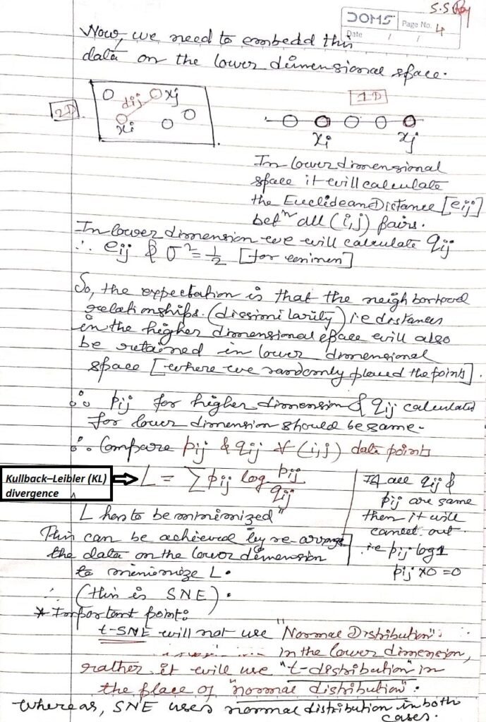
Why asymmetric KL-divergence?
→ Emphasizes preserving local neighborhoods more than global structure.
t-SNE vs. UMAP trade-offs?
→ UMAP faster, preserves global structure better than t-SNE.
Why not for downstream ML tasks?
→ Embeddings distort distances; unsuitable for predictive models.
Effect of initialization?
→ PCA gives stable maps; random can cause variability.
Scaling to millions of points?
→ Use Barnes-Hut or FFT approximations for efficiency.
Limitations of interpretability?
→ Global distances meaningless; only local clusters reliable.
Relation to manifold learning?
→ Captures local manifold structure via probabilistic similarities.
Misleading conclusions risk?
→ Wrong perplexity or iterations produce artificial clusters.
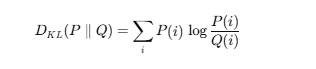
Kullback–Leibler (KL) divergence–>
Kullback–Leibler (KL) divergence is an information-theoretic measure of how a probability distribution PPP diverges from a reference distribution Q. It is asymmetric, always non-negative, and equals zero only if P=Q. Widely used in t-SNE, variational inference, and generative models, KL-divergence quantifies information loss when approximating P with Q.
MATRIX DATA CALCULATION.*